Page 131 - Statistics and Data Analysis in Geology

Statistics and Data Analysis in Geology - Chapter 5

As n becomes infinitely large, all of the fractions that contain n in their denominator
become infinitesimally small and vanish, so all terms inside parentheses simply
become equal to 1. The terms inside the brackets simplify to

P (r) = e (-AA) (5.12)
r!
Note that n, the number of drilling sites, has vanished from the equation leaving
only the discovery-well density, A, the number of discovery wells, Y, and the area,
A, of the tracts. This is an expression of the Poisson distribution, as applied to the
probability of rare, random events (discovery wells) occurring within geographic
areas. Also note that AA is simply the mean number of wells per tract, because it is
the product of the density of discovery wells times the area of a tract. In practice,
we estimate AA from the total number of discovery wells, m, and the total number
of tracts, T m
hA=- (5.13)
T
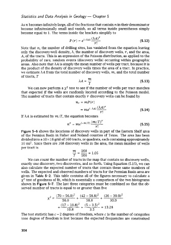
We can now perform a x2 test to see if the number of wells per tract matches
that expected if the wells are randomly located according to the Poisson model.
The number of tracts that contain exactly r discovery wells can be found by

nr = mP(r)
= me (-hA) (5.14)
r!
If AA is estimated by m/T, the equation becomes

(5.15)
Figure 5-6 shows the locations of discovery wells in part of the Eastern Shelf area
of the Permian Basin in Fisher and Noland counties of Texas. The area has been
divided into a lox 16 grid of 160 tracts, or quadrats, each containing approximately
10 mi2. Since there are 168 discovery wells in the area, the mean number of wells
per tract is
m 168
-=- = 1.05
T 160
We can count the number of tracts in the map that contain no discovery wells,
exactly one discovery, two discoveries, and so forth. Using Equation (5.15), we can
also calculate the expected number of tracts that contain these same numbers of
wells. The expected and observed numbers of tracts for the Permian Basin area are
given in Table 5-2. This table contains all of the figures necessary to calculate a
x2 test of goodness of fit, which is essentially a comparison of the two histograms
shown in Figure 5-7. The last three categories must be combined so that the ob-
served number of tracts is equal to or greater than five

70 - 56.0)’ (42 - 58.8)’ + (26 - 30.9)’
2 J +
- 56.0 58.8 30.9
+ (17 - 10.8)’ + (5 - 3.5)2 = 13.28
10.8 3.5
‘The test statistic has c - 2 degrees of freedom, where c is the number of categories
(one degree of freedom is lost because the expected frequencies are constrained

304