Page 242 - Statistics for Environmental Engineers

L1592_frame_C27.fm Page 245 Tuesday, December 18, 2001 2:47 PM

Two-factor interaction of compaction × time (X 23 ⋅ y)
107.9 + 120.8 + 107.6 + 118.9 118.6 + 126.5 + 99.8 + 117.5
------------------------------------------------------------------------- – --------------------------------------------------------------------- = – 1.80
4 4

Three-factor interaction of water × compaction × time (X 123 ⋅ y)
120.8 + 118.6 + 99.8 + 118.9 107.9 + 126.5 + 117.5 + 107.6
--------------------------------------------------------------------- – ------------------------------------------------------------------------- = – 0.35
4 4
Before interpreting these effects, we want to know whether they are large enough not to have arisen
from random error. If we had an estimate of the variance of measurement error, the variance of each
effect could be estimated and confidence intervals could be used to make this assessment. In this
experiment there are no replicated measurements, so it is not possible to compute an estimate of the
variance. Lacking a variance estimate, another approach is used to judge the significance of the effects.
If the effects are random (i.e., arising from random measurement errors), they might be expected to
be normally distributed, just as other random variables are expected to be normally distributed. Random
effects will plot as a straight line on normal probability paper. The normal plot is constructed by ordering
the effects (excluding the average), computing the probability plotting points as shown in Chapter 5,
and making a plot on normal probability paper. Because probability paper is not always handy, and
many computer graphics programs do not make probability plots, it is handy to plot the effects against
the normal order scores (or rankits). Table 27.4 shows both the probability plotting positions and the
normal order scores for the effects.
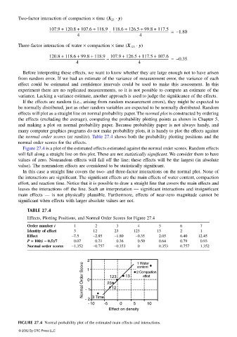
Figure 27.4 is a plot of the estimated effects estimated against the normal order scores. Random effects
will fall along a straight line on this plot. These are not statistically significant. We consider them to have
values of zero. Nonrandom effects will fall off the line; these effects will be the largest (in absolute
value). The nonrandom effects are considered to be statistically significant.
In this case a straight line covers the two- and three-factor interactions on the normal plot. None of
the interactions are significant. The significant effects are the main effects of water content, compaction
effort, and reaction time. Notice that it is possible to draw a straight line that covers the main effects and
leaves the interactions off the line. Such an interpretation — significant interactions and insignificant
main effects — is not physically plausible. Furthermore, effects of near-zero magnitude cannot be
significant when effects with larger absolute values are not.
TABLE 27.4
Effects, Plotting Positions, and Normal Order Scores for Figure 27.4
Order number i 1 2 3 4 5 6 7
Identity of effect 3 12 23 123 13 2 1
Effect −7.5 −2.85 −1.80 −0.35 2.05 6.40 12.45
P == == 100(i −− −− 0.5)/7 0.07 0.21 0.36 0.50 0.64 0.79 0.93
Normal order scores −1.352 −0.757 −0.353 0 0.353 0.757 1.352

2 1 Water
Normal Order Score -1 23 123 13 2 Compaction
content
1
effort
0
12
-2 3 Time
- 10 -5 0 5 10
Effect on density

FIGURE 27.4 Normal probability plot of the estimated main effects and interactions.
© 2002 By CRC Press LLC