Page 238 - Statistics for Environmental Engineers

L1592_frame_C27.fm Page 241 Tuesday, December 18, 2001 2:47 PM

TABLE 27.2
3 4
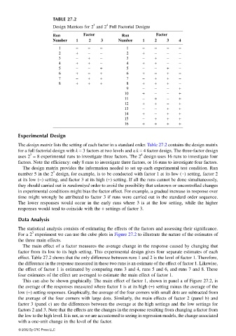
Design Matrices for 2 and 2 Full Factorial Designs
Run Factor Run Factor
Number 1 2 3 Number 1 2 3 4
1 − − − 1 − − − −
2 + − − 2 + − − −
3 − + − 3 − + − −
4 + + − 4 + + − −
5 − − + 5 − − + −
6 + − + 6 + − + −
7 − + + 7 − + + −
8 + + + 8 + + + −
9 − − − +
10 + − − +
11 − + − +
12 + + − +
13 − − + +
14 + − + +
15 − + + +
16 + + + +

Experimental Design
The design matrix lists the setting of each factor in a standard order. Table 27.2 contains the design matrix
for a full factorial design with k = 3 factors at two levels and a k = 4 factor design. The three-factor design
4
3
uses 2 = 8 experimental runs to investigate three factors. The 2 design uses 16 runs to investigate four
factors. Note the efficiency: only 8 runs to investigate three factors, or 16 runs to investigate four factors.
The design matrix provides the information needed to set up each experimental test condition. Run
3
number 5 in the 2 design, for example, is to be conducted with factor 1 at its low (−) setting, factor 2
at its low (−) setting, and factor 3 at its high (+) setting. If all the runs cannot be done simultaneously,
they should carried out in randomized order to avoid the possibility that unknown or uncontrolled changes
in experimental conditions might bias the factor effect. For example, a gradual increase in response over
time might wrongly be attributed to factor 3 if runs were carried out in the standard order sequence.
The lower responses would occur in the early runs where 3 is at the low setting, while the higher
responses would tend to coincide with the + settings of factor 3.

Data Analysis
The statistical analysis consists of estimating the effects of the factors and assessing their significance.
3
For a 2 experiment we can use the cube plots in Figure 27.2 to illustrate the nature of the estimates of
the three main effects.
The main effect of a factor measures the average change in the response caused by changing that
factor from its low to its high setting. This experimental design gives four separate estimates of each
effect. Table 27.2 shows that the only difference between runs 1 and 2 is the level of factor 1. Therefore,
the difference in the response measured in these two runs is an estimate of the effect of factor 1. Likewise,
the effect of factor 1 is estimated by comparing runs 3 and 4, runs 5 and 6, and runs 7 and 8. These
four estimates of the effect are averaged to estimate the main effect of factor 1.
This can also be shown graphically. The main effect of factor 1, shown in panel a of Figure 27.2, is
the average of the responses measured where factor 1 is at its high (+) setting minus the average of the
low (−) setting responses. Graphically, the average of the four corners with small dots are subtracted from
the average of the four corners with large dots. Similarly, the main effects of factor 2 (panel b) and
factor 3 (panel c) are the differences between the average at the high settings and the low settings for
factors 2 and 3. Note that the effects are the changes in the response resulting from changing a factor from
the low to the high level. It is not, as we are accustomed to seeing in regression models, the change associated
with a one-unit change in the level of the factor.
© 2002 By CRC Press LLC