Page 28 - Statistics for Environmental Engineers

L1592_Frame_C02 Page 19 Tuesday, December 18, 2001 1:40 PM

14 40 random samples of n = 4
Parent
y 10 distribution

N(10,1)
6
12 Sampling
y= Σy 10 distribution
n of the mean
8 is normal

6
4
2 Σ( y −y )
s = 2 2 Sampling
n−1 distribution of
0 the variance
2
t = y −η 0 Sampling
distribution
sn
of t
-2
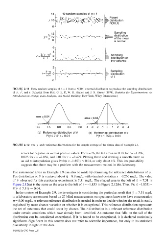
FIGURE 2.11 Forty random samples of n = 4 from a N(10,1) normal distribution to produce the sampling distributions
2
of , s , and t. (Adapted from Box, G. E. P., W. G. Hunter, and J. S. Hunter (1978). Statistics for Experimenters: An
y
Introduction to Design, Data Analysis, and Model Building, New York, Wiley Interscience.)

area = 0.04
area = 0.04

7.0 7.5 8.0 8.5 9.0 -4 -3 -2 -1 0 1 2 3 4
(a) Reference distribution of y ¯ (b) Reference distribution of t
P(y ≤ 7.51) = 0.04 P(t ≤ 1.853) = 0.04
¯
y
FIGURE 2.12 The and t reference distributions for the sample average of the nitrate data of Example 2.1.
serves for negative as well as positive values. For ν = 26, the tail areas are 0.05 for t = –1.706,
0.025 for t = –2.056, and 0.01 for t = –2.479. Plotting these and drawing a smooth curve as
an aid to interpolation gives Prob(t < –1.853) 0.04, or only about 4%. This low probability
suggests that there may be a problem with the measurement method in this laboratory.

The assessment given in Example 2.9 can also be made by examining the reference distributions of .
y
The distribution of is centered about η = 8.0 mg/L with standard deviation s = 0.266 mg/L. The valuey
y
of observed for this particular experiment is 7.51 mg/L. The shaded area to the left of = 7.51 in
y
Figure 2.12(a) is the same as the area to the left of t = –1.853 in Figure 2.12(b). Thus, P(t ≤ –1.853) =
P( ≤ 7.51) 0.04.
y
In the context of Example 2.9, the investigator is considering the particular result that = 7.51 mg/L
y
in a laboratory assessment based on 27 blind measurements on specimens known to have concentration
η = 8.00 mg/L. A relevant reference distribution is needed in order to decide whether the result is easily
explained by mere chance variation or whether it is exceptional. This reference distribution represents
the set of outcomes that could occur by chance. The t distribution is a relevant reference distribution
under certain conditions which have already been identified. An outcome that falls on the tail of the
distribution can be considered exceptional. If it is found to be exceptional, it is declared statistically
significant. Significant in this context does not refer to scientific importance, but only to its statistical
plausibility in light of the data.
© 2002 By CRC Press LLC