Page 25 - Statistics for Environmental Engineers

L1592_Frame_C02 Page 16 Tuesday, December 18, 2001 1:40 PM

α
z z

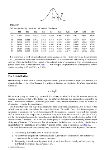
TABLE 2.1
Tail Area Probability (α) of the Unit Normal Distribution
z 0.00 0.01 0.02 0.03 0.04 0.05 0.06 0.07 0.08 0.09
0.0 0.5000 0.4960 0.4920 0.4880 0.4840 0.4801 0.4761 0.4721 0.4681 0.4641
… … … … … … … … … … …
1.5 0.0668 0.0655 0.0643 0.0630 0.0618 0.0606 0.0594 0.0582 0.0571 0.0559
1.6 0.0548 0.0537 0.0526 0.0516 0.0505 0.0495 0.0485 0.0475 0.0465 0.0455
1.7 0.0446 0.0436 0.0427 0.0418 0.0409 0.0401 0.0392 0.0384 0.0375 0.0367
1.8 0.0359 0.0351 0.0344 0.0366 0.0329 0.0322 0.0314 0.0307 0.0301 0.0294
1.9 0.0287 0.0281 0.0274 0.0268 0.0262 0.0256 0.0250 0.0244 0.0239 0.0233
2.0 0.0228 0.0222 0.0217 0.0212 0.0207 0.0202 0.0197 0.0192 0.0188 0.0183

It is convenient to work with standardized normal deviates, z = (y − η) σ, where z has the distribution
N(0, 1), because the areas under the standardized normal curve are tabulated. This merely scales the data
in terms of the standard deviation instead of the original units of measurement (e.g., concentration). A
portion of this table is reproduced in Table 2.1. For example, the probability of a standardized normal
deviate exceeding 1.57 is 0.0582, or 5.82%.

The t Distribution
Standardizing a normal random variable requires that both η and σ are known. In practice, however, we
cannot calculate z = (y − η) σ because σ is unknown. Instead, we substitute s for σ and calculate the
t statistic:
y η–
t = ------------
s
The value of η may be known (e.g., because it is a primary standard) or it may be assumed when con-
structing a hypothesis that will be tested (e.g., the difference between two treatments is assumed to be
zero). Under certain conditions, which are given below, t has a known distribution, called the Student’s t
distribution, or simply the t distribution.
The t distribution is bell-shaped and symmetric (like the normal distribution), but the tails of the
t distribution are wider than tails of the normal distribution. The width of the t distribution depends on
2
the degree of uncertainty in s , which is measured by the degrees of freedom ν on which this estimate
2 2 2 2
of s is based. When the sample size is infinite (ν = ∞), there is no uncertainty in s (because s = σ )
and the t distribution becomes the standard normal distribution. When the sample size is small (ν ≤ 30),
2
the variation in s increases. This is reflected by the spread of the t distribution increasing as the number
2
of degrees of freedom of s decreases. The tail area under the bell-shaped curve of the t distribution is
the probability of t exceeding a given value. A portion of the t table is reproduced in Table 2.2.
The conditions under which the quantity t = (y − η) s has a t distribution with ν degrees of freedom are:
2
1. y is normally distributed about η with variance σ .
2. s is distributed independently of the mean; that is, the variance of the sample does not increase
or decrease as the mean increases or decreases.
2
3. The quantity s , which has ν degrees of freedom, is calculated from normally and independently
2
distributed observations having variance σ .
© 2002 By CRC Press LLC