Page 24 - Statistics for Environmental Engineers

L1592_Frame_C02 Page 15 Tuesday, December 18, 2001 1:40 PM

11
Nitrate Observation i-1 9 8
10

7
6
5
4
4 5 6 7 8 9 10 11
Nitrate Observation i

FIGURE 2.9 Plot of measurement y i vs. measurement y i−1 shows a lack of serial correlation between adjacent measurements.

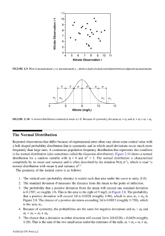
σ σ σ σ σ σ

α 1 α 2 α 3 α 4

4 6 8 10 12
Nitrate (mg/L)

FIGURE 2.10 A normal distribution centered at mean η = 8. Because of symmetry, the areas α 1 = α 4 and α 1 + α 2 = α 3 + α 4 .

The Normal Distribution
Repeated observations that differ because of experimental error often vary about some central value with
a bell-shaped probability distribution that is symmetric and in which small deviations occur much more
frequently than large ones. A continuous population frequency distribution that represents this condition
is the normal distribution (also sometimes called the Gaussian distribution). Figure 2.10 shows a normal
2
distribution for a random variable with η = 8 and σ = 1. The normal distribution is characterized
2
completely by its mean and variance and is often described by the notation N(η, σ ), which is read “a
2
normal distribution with mean η and variance σ .”
The geometry of the normal curve is as follows:
1. The vertical axis (probability density) is scaled such that area under the curve is unity (1.0).
2. The standard deviation σ measures the distance from the mean to the point of inflection.
3. The probability that a positive deviation from the mean will exceed one standard deviation
is 0.1587, or roughly 1 6. This is the area to the right of 9 mg/L in Figure 2.8. The probability
that a positive deviation will exceed 2σ is 0.0228 (roughly 1 40), which is area α 3 + α 4 in
Figure 2.8. The chance of a positive deviation exceeding 3σ is 0.0013 (roughly 1 750), which
is the area α 4 .
4. Because of symmetry, the probabilities are the same for negative deviations and α 1 = α 4 and
α 1 + α 2 = α 3 + α 4 .
5. The chance that a deviation in either direction will exceed 2σ is 2(0.0228) = 0.0456 (roughly
1 20). This is the sum of the two small areas under the extremes of the tails, α 1 + α 2 = α 3 + α 4 .

© 2002 By CRC Press LLC