Page 33 - Statistics for Environmental Engineers

L1592_Frame_C02 Page 24 Tuesday, December 18, 2001 1:40 PM

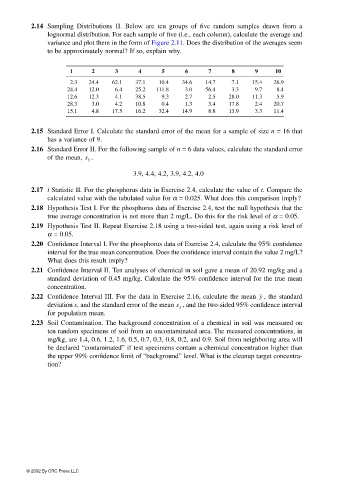
2.14 Sampling Distributions II. Below are ten groups of five random samples drawn from a
lognormal distribution. For each sample of five (i.e., each column), calculate the average and
variance and plot them in the form of Figure 2.11. Does the distribution of the averages seem
to be approximately normal? If so, explain why.

1 2 3 4 5 6 7 8 9 10
2.3 24.4 62.1 37.1 10.4 34.6 14.7 7.1 15.4 26.9
24.4 12.0 6.4 25.2 111.8 3.0 56.4 3.3 9.7 8.4
12.6 12.3 4.1 38.5 9.3 2.7 2.5 28.0 11.3 5.9
28.3 3.0 4.2 10.8 0.4 1.3 3.4 17.8 2.4 20.7
15.1 4.8 17.5 16.2 32.4 14.9 8.8 13.9 3.3 11.4

2.15 Standard Error I. Calculate the standard error of the mean for a sample of size n = 16 that
has a variance of 9.
2.16 Standard Error II. For the following sample of n = 6 data values, calculate the standard error
.
of the mean, s y
3.9, 4.4, 4.2, 3.9, 4.2, 4.0

2.17 t Statistic II. For the phosphorus data in Exercise 2.4, calculate the value of t. Compare the
calculated value with the tabulated value for α = 0.025. What does this comparison imply?
2.18 Hypothesis Test I. For the phosphorus data of Exercise 2.4, test the null hypothesis that the
true average concentration is not more than 2 mg/L. Do this for the risk level of α = 0.05.
2.19 Hypothesis Test II. Repeat Exercise 2.18 using a two-sided test, again using a risk level of
α = 0.05.
2.20 Confidence Interval I. For the phosphorus data of Exercise 2.4, calculate the 95% confidence
interval for the true mean concentration. Does the confidence interval contain the value 2 mg/L?
What does this result imply?
2.21 Confidence Interval II. Ten analyses of chemical in soil gave a mean of 20.92 mg/kg and a
standard deviation of 0.45 mg/kg. Calculate the 95% confidence interval for the true mean
concentration.
2.22 Confidence Interval III. For the data in Exercise 2.16, calculate the mean , the standard
y
deviation s, and the standard error of the mean , and the two-sided 95% confidence interval
s y
for population mean.
2.23 Soil Contamination. The background concentration of a chemical in soil was measured on
ten random specimens of soil from an uncontaminated area. The measured concentrations, in
mg/kg, are 1.4, 0.6, 1.2, 1.6, 0.5, 0.7, 0.3, 0.8, 0.2, and 0.9. Soil from neighboring area will
be declared “contaminated” if test specimens contain a chemical concentration higher than
the upper 99% confidence limit of “background” level. What is the cleanup target concentra-
tion?

© 2002 By CRC Press LLC