Page 65 - Statistics for Environmental Engineers

L1592_frame_C06 Page 57 Tuesday, December 18, 2001 1:43 PM

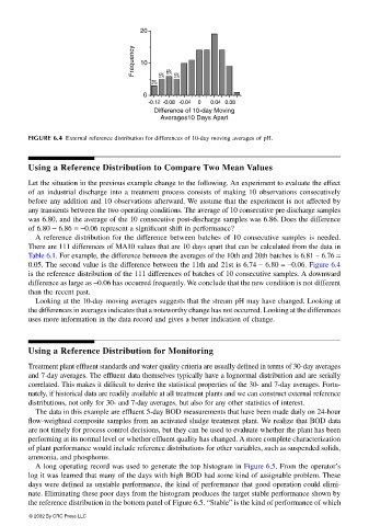
20
Frequency 10 6%

3% 5% 5%
0
-0.12 -0.08 -0.04 0 0.04 0.08
Difference of 10-day Moving
Averages10 Days Apart

FIGURE 6.4 External reference distribution for differences of 10-day moving averages of pH.

Using a Reference Distribution to Compare Two Mean Values

Let the situation in the previous example change to the following. An experiment to evaluate the effect
of an industrial discharge into a treatment process consists of making 10 observations consecutively
before any addition and 10 observations afterward. We assume that the experiment is not affected by
any transients between the two operating conditions. The average of 10 consecutive pre-discharge samples
was 6.80, and the average of the 10 consecutive post-discharge samples was 6.86. Does the difference
of 6.80 − 6.86 = −0.06 represent a significant shift in performance?
A reference distribution for the difference between batches of 10 consecutive samples is needed.
There are 111 differences of MA10 values that are 10 days apart that can be calculated from the data in
Table 6.1. For example, the difference between the averages of the 10th and 20th batches is 6.81 − 6.76 =
0.05. The second value is the difference between the 11th and 21st is 6.74 − 6.80 = −0.06. Figure 6.4
is the reference distribution of the 111 differences of batches of 10 consecutive samples. A downward
difference as large as −0.06 has occurred frequently. We conclude that the new condition is not different
than the recent past.
Looking at the 10-day moving averages suggests that the stream pH may have changed. Looking at
the differences in averages indicates that a noteworthy change has not occurred. Looking at the differences
uses more information in the data record and gives a better indication of change.

Using a Reference Distribution for Monitoring
Treatment plant effluent standards and water quality criteria are usually defined in terms of 30-day averages
and 7-day averages. The effluent data themselves typically have a lognormal distribution and are serially
correlated. This makes it difficult to derive the statistical properties of the 30- and 7-day averages. Fortu-
nately, if historical data are readily available at all treatment plants and we can construct external reference
distributions, not only for 30- and 7-day averages, but also for any other statistics of interest.
The data in this example are effluent 5-day BOD measurements that have been made daily on 24-hour
flow-weighted composite samples from an activated sludge treatment plant. We realize that BOD data
are not timely for process control decisions, but they can be used to evaluate whether the plant has been
performing at its normal level or whether effluent quality has changed. A more complete characterization
of plant performance would include reference distributions for other variables, such as suspended solids,
ammonia, and phosphorus.
A long operating record was used to generate the top histogram in Figure 6.5. From the operator’s
log it was learned that many of the days with high BOD had some kind of assignable problem. These
days were defined as unstable performance, the kind of performance that good operation could elimi-
nate. Eliminating these poor days from the histogram produces the target stable performance shown by
the reference distribution in the bottom panel of Figure 6.5. “Stable” is the kind of performance of which
© 2002 By CRC Press LLC