Page 76 - Statistics for Environmental Engineers

L1592_frame_C07.fm Page 68 Tuesday, December 18, 2001 1:44 PM

TABLE 7.6
Transformed Values, Means, and Variances as a Function of λ
λλ λλ == == −− −−1 λλ λλ == == −− −− 0.5 λλ λλ == == 0 λλ λλ == == 0.5 λλ λλ == == 1
−0.0061 −0.0146 −0.0451 −0.1855 −0.9770
−0.0070 −0.0159 −0.0467 −0.1877 −0.9800
−0.0141 −0.0235 −0.0550 −0.1967 −0.9900
… … … … …
… … … … …
−0.0284 −0.0343 −0.0633 −0.2032 −0.9950
−0.0108 −0.0203 −0.0519 −0.1937 −0.9870
λ
y = −0.01496 0.0228 − −0.0529 −0.1930 −0.9839
λ
Var y () = 0.000093 0.000076 0.000078 0.000113 0.000255

0. 3
Variance (x1000) 0. 2 log transformation No transformation

1
0.
0. 0
-1.0 -0.5 0.0 0.5 1.0
λ

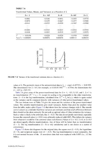
FIGURE 7.4 Variance of the transformed cadmium data as a function of λ.

values of λ. The geometric mean of the untransformed data is y = exp – ( 4.42723) = 0.01195.
g
0.5−1
The denominator for λ = 0.5, for example, is 0.5(0.01195) = 4.5744; the denominator for
λ = −0.5 is −765.747.
Table 7.6 gives some of the power-transformed data for λ = −1, −0.5, 0, 0.5, and 1. λ = 1 is
no transformation Y i =( 1 () y i – 1) except for scaling to be comparable to the other transforma-
0 () =
g
tions. λ = 0 is the log transformation, calculated from Y i y ln (), which is again scaled
y i
so the variance can be compared directly with variances of other power-transformed values.
The two bottom rows of Table 7.6 give the mean and the variance of the power-transformed
values. The suitable transformations give small variances. Rather than pick the smallest value
from the table, make a plot (Figure 7.4) that shows how the variance changes with λ. The smooth
curve is drawn as a reminder that these variances are estimates and that small differences between
them should not be taken seriously. Do not seek an optimal value of λ that minimizes the variance.
Such a value is likely to be awkward, like λ = 0.23. The data do not justify such detail, especially
because the censored values (y < 0.01) were arbitrarily replaced with 0.005. (This inflates the variance
from whatever it would be if the censored values were known.) Values of λ = −0.5, λ = 0, or λ = 0.5
are almost equally effective transformations. Any of these will be better than no transformation
(λ = 1). The log transformation (λ = 0) is very satisfactory and is our choice as a matter of
convenience.
Figure 7.5 shows dot diagrams for the original data, the square root (λ = 0.5), the logarithms
(λ = 0), and reciprocal square root (λ = −0.5). The log transformation is most symmetric, but
it is not normal because of the 11 non-detect data that were replaced with 0.005 (i.e., 1/2 the
MDL).

© 2002 By CRC Press LLC