Page 74 - Statistics for Environmental Engineers

L1592_frame_C07.fm Page 66 Tuesday, December 18, 2001 1:44 PM

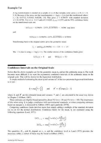
Example 7.4

A log transformation is needed on a sample of n = 6 that includes some zeros: y = [0, 2, 1, 0,
3, 9]. Because of the zeros, use the transformation x = log(y + 1) to find the transformed values:
x = [0, 0.47712, 0.30103, 0.60206, 1.0]. This gives x = 0.39670 with standard deviation
2
s x = 0.14730. For ν = n − 1 = 5 and α/2 = 0.025, t 5,0.025 = 2.571 and the 95% confidence limits
on the transformed scale are:
LCL x() = 0.39670 2.571 0.14730/6 = – 0.006 (say zero)
–
and

UCL x() = 0.39670 + 2.571 0.14730/6 = 0.79954

Transforming back to the original metric gives the geometric mean:

y = antilog 10 0.39670) 1 = 2.5 1 = 1.5
(
–
–
g
The −1 is due to using x = log(y + 1). The similar inverse of the confidence limits gives:
LCL y() = 0 and UCL y() = 5.3

Confidence Intervals on the Original Scale
Notice that the above examples are for the geometric mean η g and not the arithmetic mean η. The work
becomes more difficult if we want the asymmetric confidence intervals of the arithmetic mean on the
original scale. This will be shown for the lognormal distribution.
2
A simple method of estimating the mean η and variance σ of the two-parameter lognormal distribution
is to use:

2

η ˆ = exp x + s x and σ ˆ = η ˆ exp () 1]
[
2
2
2
----
–

2 
s x
x
η ˆ
where and σ ˆ 2 are the estimated mean and variance. and s x 2 are calculated in the usual way shown
in Chapter 2 (Gilbert, 1987).
These estimates are slightly biased upward by about 5% for n = 20 and 1% for n = 100. The importance
η ˆ
of this when using to judge compliance with environmental standards, or when comparing estimates
based on unequal n, is discussed by Gilbert (1987) and Landwehr (1978).
Computing confidence limits involves more than simply adding a multiple of the standard deviation
(as we do for the normal distribution). Confidence limits for the mean, η, are estimated using the
following equations (Land, 1971):
=  x + 0.5s x + s y H 1 α– 
2
UCL 1 α– exp  ----------------- 
–
n 1
s y H α 
LCL α = exp   x + 0.5s x + ---------------- 
2
–
n 1
The quantities H 1–α and H α depend on s x , n, and the confidence level α. Land (1975) provides the
necessary tables; a subset of these may be found in Gilbert (1987).
© 2002 By CRC Press LLC