Page 73 - Statistics for Environmental Engineers

L1592_frame_C07.fm Page 65 Tuesday, December 18, 2001 1:44 PM

Confidence Intervals and Transformations
After summary statistics (means, standard deviations, etc.) have been calculated on the transformed
scale, it is often desirable to translate the results back to the original scale of measurement. This can
x
create some confusion. For example, if the average has been estimated using x = log(y), the simple
x
x
back-transformation of antilog( ) does not give an unbiased estimate of y. The antilogarithm of is
x
the geometric mean of the original data (y); that is, antilog( ) = y g . The correct estimate of the arithmetic
mean on the original y scale is = antilog( + 0.5 s ) (Gilbert, 1987).y x 2
If the transformation produced a near-normal distribution, the standard deviations and standard errors
computed from the transformed data will be symmetric about the mean on the transformed scale. But
they will be asymmetric on the original scale. The options are to:
1. Quote symmetric confidence limits on the transformed scale.
2. Quote asymmetric confidence limits on the original scale (recognizing that in the case of a
log transformation they apply to the geometric mean and not to the arithmetic average).
3. Give two sets of results, one with standard errors and symmetric confidence limits on the
transformed scale and a corresponding set of means (arithmetic and geometric) on the original
scale. The reader can judge the statistical significance on the transformed scale and the
practical importance on the original scale.

Two examples illustrate the use of log-transformed data to construct confidence limits for the geometric
mean.

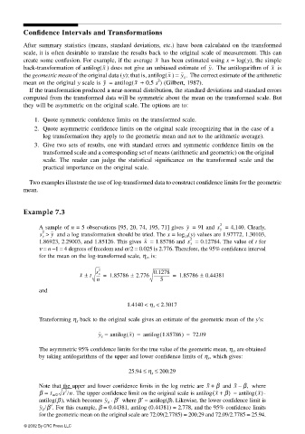
Example 7.3

y 2 = 4,140. Clearly,
A sample of n = 5 observations [95, 20, 74, 195, 71] gives = 91 and s y
s y > y and a log transformation should be tried. The x = log 10 (y) values are 1.97772, 1.30103,
2
x 2 = 0.12784. The value of t for
1.86923, 2.29003, and 1.85126. This gives = 1.85786 and s x
ν = n − 1 = 4 degrees of freedom and α/2 = 0.025 is 2.776. Therefore, the 95% confidence interval
for the mean on the log-transformed scale, η x , is:
2
x t ----± s x = 1.85786 2.776 ----------------± 0.1278 = 1.85786 0.44381
±
n 5
and

1.4140 < η x < 2.3017

Transforming η x back to the original scale gives an estimate of the geometric mean of the y’s:
(
y g = antilog x () = antilog 1.85786) = 72.09

The asymmetric 95% confidence limits for the true value of the geometric mean, η x , are obtained
by taking antilogarithms of the upper and lower confidence limits of η x , which gives:
25.94 ≤ η g ≤ 200.29

Note that the upper and lower confidence limits in the log metric are x + β and x β– , where
2
β = t α/2 s /n. The upper confidence limit on the original scale is antilog x +( β) = antilog x () ⋅
antilog(β), which becomes y g β′ where β′ = antilog(β). Likewise, the lower confidence limit is
⋅
y g/β′. For this example, β = 0.44381, antilog (0.44381) = 2.778, and the 95% confidence limits
for the geometric mean on the original scale are 72.09(2.7785) = 200.29 and 72.09/2.7785 = 25.94.
© 2002 By CRC Press LLC