Page 301 - Sustainability in the Process Industry Integration and Optimization

278 C h apter Ele v e n

Given the list of potential activities defined by their preconditions
(activating entities) and effects (resulting entities), the Maximal
Structure Generation (MSG) algorithm then produces the maximal
structure (Friedler et al., 1993). Next, when applied to the maximal
structure so derived, the Solution Structures Generation (SSG)
algorithm (Friedler et al., 1995) enumerates 15 combinatorially
feasible business process structures for the problem.
To determine the optimal business practice, the following
quantitative information is provided in addition to the case study’s
15 structural alternatives. The required volume of the demand is
20,000 pieces annually. Producing one piece of commodity C requires
the availability of one piece of part A and one of part B. At most 5000
pieces of part A are available at location L4 for €230 each. An
unlimited number of part A can be purchased at location L3 for €250
each, and an unlimited number of part B can be purchased at
location L2 for €310 each.
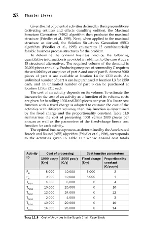
The cost of an activity depends on its volume. To estimate the
increase in the cost of an activity as a function of its volume, costs
are given for handling 1000 and 2000 pieces per year. If a linear cost
function with a fixed charge is adopted to estimate the cost of the
activities with different volumes, then this function is determined
by the fixed charge and the proportionality constant. Table 11.8
summarizes the cost of processing 1000 versus 2000 pieces per
annum as well as the parameters of the fixed-charge linear cost
function for each activity.
The optimal business process, as determined by the Accelerated
Branch-and-Bound (ABB) algorithm (Friedler et al., 1996), corresponds
to the activities given in Table 11.9 whose annual cost totals

Activity Cost of processing Cost function parameters
ID 1000 pcs/y 2000 pcs/y Fixed charge Proportionality
[€/y] [€/y] [€/y] constant
[€/pcs/y]
P 8,000 10,000 6,000 2
L1
P 9,000 10,000 8,000 1
L2
T 4,000 8,000 0 4
AL3L1
T 10,000 20,000 0 10
AL3L2
T 12,000 24,000 0 12
AL4L1
T 2,000 4,000 0 2
AL4L2
T 10,000 20,000 0 10
BL2L1
T 14,000 28,000 0 14
CL2L1
TABLE 11.8 Cost of Activities in the Supply Chain Case Study