Page 105 - The Geological Interpretation of Well Logs

- SONIC OR ACOUSTIC LOGS -

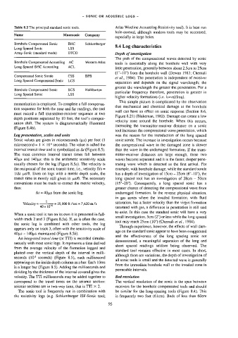
Table 8.2 The principal standard sonic tools. Atlas Wireline Acoustilog-Resistivity tool). It is best run

hole-centred, although modern tools may be eccentred,
Name Mnemonic Company
especially in large holes.

Borehole Compensated Sonic BHC Schlumberger
8.4 Log characteristics
Long Spaced Sonic LSS
Astay-Sonic (standard made) DTCO Depth of investigation

The path of the compressional waves detected by sonic
Borehole Compensated Acoustilog AC Western Atlas
tools is essentially along the borehole wall with very
Long Spaced BHC Acoustilog ACL
little penetration, generally between about 2.5cm to 25cm

(1"-10") from the borehole wall (Dewan 1983; Chemali
Compensated Sonic Sonde css BPB
ét-al., 1984). The penetration is independent of receiver
Long Spaced Compensated Sonic LCS
separation and depends on the signal wavelength; the

greater the wavelength the greater the penetration, For a
Borehole Compensated Sonic BCS Halliburton
particular frequency therefore, penetration is greater in
Long Spaced Sonic LSS
higher velocity formations (i.e. A=vel/freq).

This simple picture is complicated by the observation
memorisation is employed. To complete a full compensa-
that mechanical and chemical damage at the borehole
tion sequence for both the near and far readings, the tool
wall can have an effect on sonic response (Section 8.6,
must record a full transmitter-receiver sequence at two
Figure 8.21) (Blakeman, 1982). Damage can create a low
depth positions separated by 10 feet, the tool’s compen-
velocity zone around the borehole. When this occurs,
sation shift. The system is diagrammatically illustrated
increasing the transmitter-receiver distance on a sonic
(Figure 8.4b).
tool increases the compressional wave penetration, which
Log presentation, scales and units was the reason for the introduction of the long spaced
Sonic values are given in microseconds (js) per foot (1 sonic sonde. The increase in investigation occurs because
microsecond = | X 10 seconds). The value is calied the the compressional wave in the damaged zone is slower
interval transit time and is symbolized as Ar (Figure 8.5). than the wave in the undamaged formation. If the trans-
The most common interval transit mes fall between milter-receiver distances are large enough, these two
40s and 140s: this is the arithmetic sensitivity scale waves become separated and it is the faster, deeper pene-
usually chosen for the log (Figure 8.5a). The velocity is trating wave which is detected as the first arrival. For
the reciprocal of the sonic transit time, i.e., velocity ft/s = example, with borehole damage, while the standard sonde
I/At ps/ft. Even on logs with a metric depth scale, the has a depth of investigation of 1Scm — 25cm (6’°—10"), the
transit time is mostly still given in ys/ft. The necessary long spaced tool has an investigation of 38cm — 50cm
conversions must be made to extract the metric velocity, (LS"-20"), Consequently, a long spaced sonic has a
thus: greater chance of detecting the compressional wave from
At = 40s from the sonic log. undamaged formation. In the reverse physical situation,
in gas zones where the invaded formation, with fluid
saturation, has a faster velocity than the virgin formation
Velocity = — 25,000 ft /sec = 7,620 m/s
40x 10 saturated with gas, a difference in penetration is stil] said
to exist. In this case the standard sonic will have a very
When a sonic tool is run on its own it is presented in full-
small investigation, 5cm (2") or less while the long spaced
width track 2 and 3 (Figure 8.5a). If, as is often the case,
tool may reach 25cm (10") (Chemali et a/., 1984).
the sonic log is combined with other tools, the log
Through experience, however, the effects of wall dam-
appears only on track 3, often with the sensitivity scale of
age on the standard sonic appear to have been exaggerated
401s — 140,15 maintained (Figure 8.55).
and the effectiveness of the long spacing sonic not
An integrated travel time (or TTI) is recorded simulta-
demonstrated, a meaningful separation of the long and
neously with most sonic logs. It represents a time derived
short spaced readings seldom being observed. The
from the average velocity of the formation logged and
standard too] remains effective in most cases. In short,
plotted over the vertical depth of the interval in milli-
although there are variations, the depth of investigation of
seconds (107 seconds) (Figure 8.5), each millisecond
all sonic tools is smal] and the detected wave is generally
appearing on the inside depth column as a bar. Each 1Oms
frorn the immediate borehole wall or the invaded zone in
is a longer bar (Figure 8.5). Adding the milliseconds and
permeable intervals.
dividing by the thickness of the interval covered gives the
velocity. The TTI milliseconds may be added together to Bed resolution
correspond to the travel times on the seismic section: The vertical resolution of the sonic is the span between
seismic sections are in two-way time, that is TTI X 2. receivers for the borehole compensated tools and should
The sonic tool is frequently run in combination with be similar for the long-spacing tools (Figure 8.4). This
the resistivity logs (e.g. Schlumberger ISF-Sonic tool; is frequently two feet (61cm). Beds of less than 60cm
95