Page 135 - The Mechatronics Handbook

Known force applied to a system Known velocity input on one side and an
attachment point with zero velocity
on other

Force, F(t) V(t)
System System

ground

F(t) V(t)
S System S System
e
f
F, force back to ground
V = 0
S f
(a) (b)
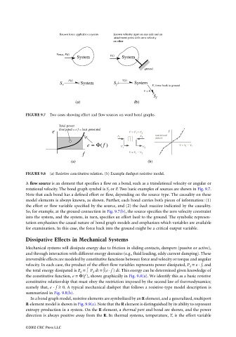
FIGURE 9.7 Two cases showing effort and flow sources on word bond graphs.

Total power
e dissipated = e f = heat generated F = F 1 = F 2 F
translational
F 1 F 2
dashpot
e = Φ( f ) V 1 V 2 V = V 1 V 2
−
−
f V = V 1 V 2
(a) (b)

FIGURE 9.8 (a) Resistive constitutive relation. (b) Example dashpot resistive model.
A flow source is an element that specifies a flow on a bond, such as a translational velocity or angular or
rotational velocity. The bond graph symbol is S f or F. Two basic examples of sources are shown in Fig. 9.7.
Note that each bond has a defined effort or flow, depending on the source type. The causality on these
model elements is always known, as shown. Further, each bond carries both pieces of information: (1)
the effort or flow variable specified by the source, and (2) the back reaction indicated by the causality.
So, for example, at the ground connection in Fig. 9.7(b), the source specifies the zero velocity constraint
into the system, and the system, in turn, specifies an effort back to the ground. The symbolic represen-
tation emphasizes the causal nature of bond graph models and emphasizes which variables are available
for examination. In this case, the force back into the ground might be a critical output variable.

Dissipative Effects in Mechanical Systems

Mechanical systems will dissipate energy due to friction in sliding contacts, dampers (passive or active),
and through interaction with different energy domains (e.g., fluid loading, eddy current damping). These
irreversible effects are modeled by constitutive functions between force and velocity or torque and angular
velocity. In each case, the product of the effort-flow variables represents power dissipated, P d = e · f, and
the total energy dissipated is E d = ∫ P d dt = ∫(e · f ) dt. This energy can be determined given knowledge of
the constitutive function, e = Φ(f ), shown graphically in Fig. 9.8(a). We identify this as a basic resistive
constitutive relationship that must obey the restriction imposed by the second law of thermodynamics;
namely that, e · f ≥ 0. A typical mechanical dashpot that follows a resistive-type model description is
summarized in Fig. 9.8(b).
In a bond graph model, resistive elements are symbolized by an R element, and a generalized, multiport
R-element model is shown in Fig. 9.9(a). Note that the R element is distinguished by its ability to represent
entropy production in a system. On the R element, a thermal port and bond are shown, and the power
direction is always positive away from the R. In thermal systems, temperature, T, is the effort variable

©2002 CRC Press LLC