Page 133 - The Mechatronics Handbook

F 1 F 2
e 1 device
f 1
V 1 V 2
e 2 e n
0 F =F = F
f 2 f n 1 2 3
e 3 F 1 F 2
1 0 1
f 3
V 1 V 2
f + f + f +(etc.)+ f = 0 F 3 V 3 V − V = V
1 2 3 n 1 2 3
spring 1
e = e = e = (etc.)= e Same velocity
1 2 3 n V spring
(a) (b)

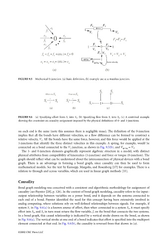
FIGURE 9.5 Mechanical 0-junction: (a) basic definition, (b) example use at a massless junction.

S S
Effort into S Flow into S 2 3
2 2
e e
S S S S
1 f 2 1 f 2 S S
1 1 0 4
(a) (b) (c)

FIGURE 9.6 (a) Specifying effort from S 1 into S 2 . (b) Specifying flow from S 1 into S 2 . (c) A contrived example
showing the constraint on causality assignment imposed by the physical definitions of 0- and 1-junctions.

on each end is the same (note this assumes there is negligible mass). The definition of the 0-junction
implies that all the bonds have different velocities, so a flow difference can be formed to construct a
relative velocity, V 3 . All the bonds have the same force, however, and this force would be applied at the
1-junctions that identify the three distinct velocities in this example. A spring, for example, would be
connected on a bond connected to the V 3 junction, as shown in Fig. 9.5(b), and V spring = V 3 .
The 1- and 0-junction elements graphically represent algebraic structure in a model, with distinct
physical attributes from compatibility of kinematics (1-junction) and force or torque (0-junction). The
graph should reflect what can be understood about the interconnection of physical devices with a bond
graph. There is an advantage in forming a bond graph, since causality can then be used to form
mathematical models. See the text by Karnopp, Margolis, and Rosenberg [17] for examples. There is a
relation to through and across variables, which are used in linear graph methods [33].

Causality
Bond graph modeling was conceived with a consistent and algorithmic methodology for assignment of
causality (see Paynter [28], p. 126). In the context of bond graph modeling, causality refers to the input–
output relationship between variables on a power bond, and it depends on the systems connected to
each end of a bond. Paynter identified the need for this concept having been extensively involved in
analog computing, where solutions rely on well-defined relationships between signals. For example, if
system S 1 in Fig. 9.6(a) is a known source of effort, then when connected to a system S 2 , it must specify
effort into S 2 , and S 2 in turn must return the flow variable, f, on the bond that connects the two systems.
In a bond graph, this causal relationship is indicated by a vertical stroke drawn on the bond, as shown
in Fig. 9.6(a). The vertical stroke at one end of a bond indicates that effort is specified into the multiport
element connected at that end. In Fig. 9.6(b), the causality is reversed from that shown in (a).

©2002 CRC Press LLC