Page 132 - The Mechatronics Handbook

Interconnection of Components

In this chapter, we will use bond graphs to model mechanical systems. Like other graph representations
used in system dynamics [33] and multibody system analysis [30,39], bond graphs require an under-
standing of basic model elements used to represent a system. However, once understood, graph methods
provide a systematic method for representing the interconnection of multi-energetic system elements.
In addition, bond graphs are unique in that they are not linear graph formulations: power bonds replace
branches, multiports replace nodes [28]. In addition, they include a systematic approach for computa-
tional causality.
Recall that a single line represents power flow, and a half-arrow is used to designate positive power
flow direction. Nodes in a linear graph represent across variables (e.g., velocity, voltage, flowrate);
however, the multiport in a bond graph represents a system element that has a physical function defined
by an energetic basis. System model elements that represent masses, springs, and other components are
discussed in the next section. Two model elements that play a crucial role in describing how model
elements are interconnected are the 1-junction and 0-junction. These are ideal (power-conserving)
multiport elements that can represent specific physical relations in a system that are useful in intercon-
necting other model elements.
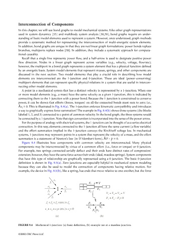
A point in a mechanical system that has a distinct velocity is represented by a 1-junction. When one
or more model elements (e.g., a mass) have the same velocity as a given 1-junction, this is indicated by
connecting them to the 1-junction with a power bond. Because the 1-junction is constrained to conserve
power, it can be shown that efforts (forces, torques) on all the connected bonds must sum to zero; i.e.,
Âe i = 0. This is illustrated in Fig. 9.4(a). The 1-junction enforces kinematic compatibility and introduces
a way to graphically express force summation! The example in Fig. 9.4(b) shows three systems (the blocks
labeled 1, 2, and 3) connected to a point of common velocity. In the bond graph, the three systems would
be connected by a 1-junction. Note that sign convention is incorporated into the sense of the power arrow.
For the purpose of analogy with electrical systems, the 1-junction can be thought of as a series electrical
connection. In this way, elements connected to the 1-junction all have the same current (a flow variable)
and the effort summation implied in the 1-junction conveys the Kirchhoff voltage law. In mechanical
systems, 1-junctions may represent points in a system that represent the velocity of a mass, and the effort
summation is a statement of Newton’s law (in D’Alembert form), ÂF - = 0.p ˙
Figure 9.4 illustrates how components with common velocity are interconnected. Many physical
components may be interconnected by virtue of a common effort (i.e., force or torque) or 0-junction.
For example, two springs connected serially deflect and their ends have distinct rates of compression/
extension; however, they have the same force across their ends (ideal, massless springs). System components
that have this type of relationship are graphically represented using a 0-junction. The basic 0-junction
definition is shown in Fig. 9.5(a). Zero junctions are especially helpful in mechanical system modeling
because they can also be used to model the connection of components having relative motion. For
example, the device in Fig. 9.5(b), like a spring, has ends that move relative to one another, but the force

e 1
f 1 V
F 1
1
e 2 e n 3
1 2 F 3
f 2 f n F 2
V = V = V = V
e 3 1 2 3
F + F − F = 0
f 3
1 2 3
f = f = f =(etc.)= f
1 2 3 n F 1 F 3
1 V 3
V 1
e + e + e + (etc.)+ e = 0 F 2 V 2
1
2
3
n
(a) (b)
FIGURE 9.4 Mechanical 1-junction: (a) basic definition, (b) example use at a massless junction.
©2002 CRC Press LLC