Page 131 - The Mechatronics Handbook

While it is convenient to use power and energy in formulating system models for mechanical systems,
a motional basis is critical for identifying interconnections and when formulating quantifiable mathe-
matical models. For many mechanical, translational, and rotational systems, it is sufficient to rely on
basic one-dimensional motion and relative motion concepts to identify the interrelation between many
types of practical components. Identifying network-like structure in these systems has been the basis for
building electrical analogies for some time. These methods, as well as signal-flow analysis techniques,
are not presented here but are the method of choice in some approaches to system dynamics [33]. Bond
graph models are presented, and it will be shown in later sections how these are consistent even with
more complex mechanical system formulations of three-dimensional dynamics as well as with the use
of Lagrangian models.

Need for Motional Basis
In modeling mechanical translational or rotational systems, it is important to identify how the configu-
ration changes, and a coordinate system should be defined and the effect of geometric changes identified.
It is assumed that the reader is familiar with these basic concepts [12]. Usually a reference configuration
is defined from which coordinates can be based. This is essential even for simple one-dimensional
translation or fixed-axis rotation. The minumum number of geometrically independent coordinates
required to describe the configuration of a system is traditionally defined as the degrees of freedom.
Constraints should be identified and can be used to choose the most convenient set of coordinates for
description of the system. We distinguish between degrees of freedom and the minimum number of
dynamic state variables that might be required to describe a system. These may be related, but they are
not necessarily the same variables or the same in number (e.g., a second-order system has two states but
is also referred to as a single degree of freedom system).
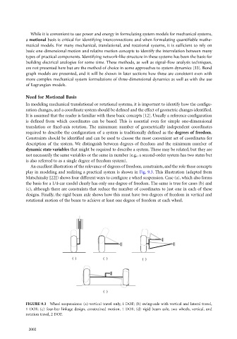
An excellent illustration of the relevance of degrees of freedom, constraints, and the role these concepts
play in modeling and realizing a practical system is shown in Fig. 9.3. This illustration (adapted from
Matschinsky [22]) shows four different ways to configure a wheel suspension. Case (a), which also forms
the basis for a 1/4-car model clearly has only one degree of freedom. The same is true for cases (b) and
(c), although there are constraints that reduce the number of coordinates to just one in each of these
designs. Finally, the rigid beam axle shows how this must have two degrees of freedom in vertical and
rotational motion of the beam to achieve at least one degree of freedom at each wheel.

(a) (b) (c)

(d)

FIGURE 9.3 Wheel suspensions: (a) vertical travel only, 1 DOF; (b) swing-axle with vertical and lateral travel,
1 DOF; (c) four-bar linkage design, constrained motion, 1 DOF; (d) rigid beam axle, two wheels, vertical, and
rotation travel, 2 DOF.

©2002 CRC Press LLC