Page 137 - The Mechatronics Handbook

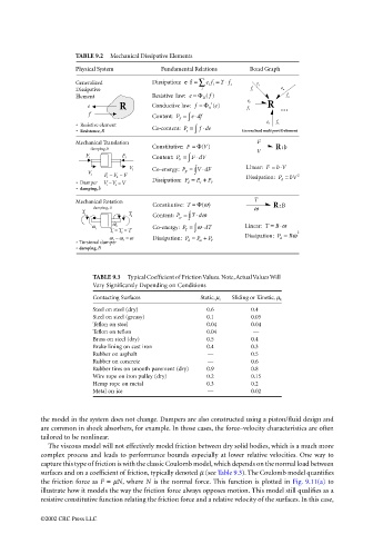
TABLE 9.2 Mechanical Dissipative Elements
Physical System Fundamental Relations Bond Graph
⋅
ef
Generalized Dissipation: ⋅= ∑ ef = T f s 1 e
ii
Dissipative i 1 f n e
f
Element Resistive law: e =Φ R ( ) n f
R R 2 f ...
e
e Conduc tive law: f =Φ − 1 ( ) 2 e R
f Content: P = e df
⋅
f ∫
3 e 3 f
Resistive element
⋅
e ∫
Resistance, R Co-content: P = f de Generalized multiport R-element
Mechanical Translation F
V
damping, b Constitutive: F =Φ ( ) V R:b
1 F 2 F Content: P = F dV
V ∫
⋅
b V
2 V Co-energy: P = V dF Linear: F =⋅
⋅
F ∫
1 V 1 F = 2 F = F Dissipation: d P = bV 2
Damper 1 VV = Dissipation: P = P + P F
2 V
V
−
d
damping, b
Mechanical Rotation T
ω
damping, B Constitutive: T =Φ ( ) ω R:B
1 T 2 T Content: P = T dω
ω ∫
⋅
⋅
1 ω 2 ω Co-energy: P = ω ⋅ dT Linear: T = B ω
T ∫
1 TT= 2 T= 2
Dissipation: P = Bω
1 ω =
ω − ω Dissipation: d P = P ω + T P d
Torsional damper 2
damping, B
TABLE 9.3 Typical Coefficient of Friction Values. Note, Actual Values Will
Vary Significantly Depending on Conditions
Contacting Surfaces Static, µ s Sliding or Kinetic, µ k
Steel on steel (dry) 0.6 0.4
Steel on steel (greasy) 0.1 0.05
Teflon on steel 0.04 0.04
Teflon on teflon 0.04 —
Brass on steel (dry) 0.5 0.4
Brake lining on cast iron 0.4 0.3
Rubber on asphalt — 0.5
Rubber on concrete — 0.6
Rubber tires on smooth pavement (dry) 0.9 0.8
Wire rope on iron pulley (dry) 0.2 0.15
Hemp rope on metal 0.3 0.2
Metal on ice — 0.02
the model in the system does not change. Dampers are also constructed using a piston/fluid design and
are common in shock absorbers, for example. In those cases, the force–velocity characteristics are often
tailored to be nonlinear.
The viscous model will not effectively model friction between dry solid bodies, which is a much more
complex process and leads to performance bounds especially at lower relative velocities. One way to
capture this type of friction is with the classic Coulomb model, which depends on the normal load between
surfaces and on a coefficient of friction, typically denoted µ (see Table 9.3). The Coulomb model quantifies
the friction force as F = µN, where N is the normal force. This function is plotted in Fig. 9.11(a) to
illustrate how it models the way the friction force always opposes motion. This model still qualifies as a
resistive constitutive function relating the friction force and a relative velocity of the surfaces. In this case,
©2002 CRC Press LLC