Page 142 - The Mechatronics Handbook

T G

V 2

T 1 w 1 V 1
w 2 T 2
F 1
F 2
i
F 1 F 2
V 2 T
v
w
V 1

V 1
i 1
V 2
F 1
v 1
P 2
F 2
Q 2
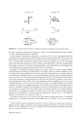
FIGURE 9.14 Common devices that can be modeled as transformers and gyrators in mechatronic systems.
the power-conserving transformation in devices for which a cross-relationship between power variables
(i.e., effort related to flow) has been identified. 2
Some examples of transformers and gyrators are shown in Fig. 9.14. In a bond graph model, the
transformer can be represented by a TF or T, while a gyrator is represented by a GY or G (note, the two
letter symbol is common). The devices shown in Fig. 9.14 indicate a modulus m or r, which may or may
not be a constant value. Many devices may have power-conserving attributes; however, the relationship
between the effort-flow variables may not be constant, so the relationship is said to be modulated when
the modulus is a function of a dynamic variable (preferably a state of the system). On a bond graph, this
can be indicated using a signal bond directed into the T or G modulus.
Examples of a modulated transformer and gyrator are given in Fig. 9.15. These examples highlight
useful techniques in modeling of practical devices. In the slider crank, note that the modulation is due
to a change in the angular position of the crank. We can get this information from a bond that is adjacent
to the transformer in question; that is, if we integrate the angular velocity found on a neighboring bond,
as shown in Fig. 9.15(a). For the field excited dc motor shown in Fig. 9.15(b), the torque–current relation
in the motor depends on a flux generated by the field; however, this field is excited by a circuit that is
powered independent of the armature circuit. The signal information for modulation does not come from
a neighboring bond, as in the case for the slider crank. These two examples illustrate two ways that
constraints are imposed in coupling mechanisms. The modulation in the slider crank might be said to
represent a holonomic constraint, and along these same lines the field excitation in the motor imposes
a non-holonomic constraint. We cannot relate torque and current in the latter case without solving for
the dynamics of an independent system—the field circuit. In the slider crank, the angular position
˙
required for the modulation is obtained simply by integrating the velocity, since = ω. Additionalq
discussion on constraints can be found in section 9.7.
The system shown in Fig. 9.16(a) is part of an all-mechanical constant-speed drive. A mechanical
feedback force, F 2 , will adjust the position of the middle rotor, x 2 . The effect is seen in the bond graph
2 It turns out that the gyrator model element is essential in all types of systems. The need for such an element to

represent gyroscopic effects in mechanical systems was first recognized by Thomson and Tait in the late 1900s.
However, it was G. D. Birkhoff (1927) and B. D. H. Tellegen (1948) who independently identified the need for this
element in analysis and synthesis of systems.

©2002 CRC Press LLC