Page 145 - The Mechatronics Handbook

i 1 v 1 .. r T 2
() =
ω 2 T 2 i G ω Zs sJ 2
2
v 1 2
1
v 1 r 2
2
() =
Zs r Y 2 () =
s
1
T 2 = r v 1 = r J 2 i 1 sJ 2
i ω
1 2
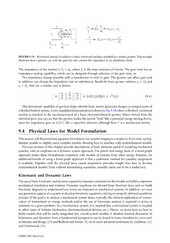
FIGURE 9.19 Rotational inertial attached to a basic rotational machine modeled as a simple gyrator. This example
illustrates how a gyrator can scale the gain but also convert the impedance to an admittance form.
The impedance of the inertial is Z 2 = sJ 2 , where J 2 is the mass moment of inertia. The gear train has an
impedance-scaling capability, which can be designed through selection of the gear ratio, m.
The impedance change possible with a transformer is only in gain. The gyrator can affect gain and
in addition can change the impedance into an admittance. Recall the basic gyrator relation, e 1 = rf 2 and
e 2 = rf 1 , then for a similar case as before,

1 e 1 f 2 e 2 2
(
= ---- ---- ---- = r [] Y 2 s()[ ] r[] = r Y 2 s (9.4)
f 1 f 2 e 2 f 1
This functional capability of gyrators helps identify basic motor-generator designs as integral parts of
a flywheel battery system. A very simplified demonstration is shown in Fig. 9.19, where a flywheel (rotational
inertia) is attached to the mechanical port of a basic electromechanical gyrator. When viewed from the
electrical port, you can see that the gyrator makes the inertia “look” like a potential energy storing device,
since the impedance goes as 1/(sC), like a capacitive element, although here C is a mechanical inertia.

9.4 Physical Laws for Model Formulation

This section will illustrate basic equation formulation for systems ranging in complexity from mass-spring-
damper models to slightly more complex models, showing how to interface with nonmechanical models.
Previous sections of this chapter provide descriptions of basic elements useful in modeling mechanical
systems, with an emphasis on a dynamic system approach. The power and energy basis of a bond graph
approach makes these formulations consistent with models of systems from other energy domains. An
additional benefit of using a bond graph approach is that a systematic method for causality assignment
is available. Together with the physical laws, causal assignment provides insight into how to develop
computational models. Even without formulating equations, causality turns out to be a useful tool.

Kinematic and Dynamic Laws

The use of basic kinematic and dynamic equations imposes a structure on the models we build to represent
mechanical translation and rotation. Dynamic equations are derived from Newton’s laws, and we build
free-body diagrams to understand how forces are imposed on mechanical systems. In addition, we must
use geometric aspects of a system to develop kinematic equations, relying on properly defined coordinate
systems. If the goal is to analyze a mechanical system alone, typically the classical application of conser-
vation of momentum or energy methods and/or the use of kinematic analysis is required to arrive at
solutions to a given problem. In a mechatronic system, it is implied that a mechanical system is coupled
to other types of systems (hydraulics, electromechanical devices, etc.). Hence, we focus here on how to
build models that will be easily integrated into overall system models. A detailed classical discussion of
kinematics and dynamics from a fundamental perspective can be found in many introductory texts such
as Meriam and Kraige [23] and Bedford and Fowler [5], or in more advanced treatments by Goldstein [11]
and Greenwood [12].

©2002 CRC Press LLC