Page 150 - The Mechatronics Handbook

directly to the mass. A free-body diagram in part (b) shows the forces exerted on the system. The spring
and damper exert forces F k and F b on the mass, and these same forces are also exerted on the fixed base
since the spring and damper are assumed to be massless. A component of the weight, W, resolved along
the axis of motion is included. The sum of applied forces is then, ∑F = F(t) + W - F k - F b . The dashed
arrow indicates the “inertial force” which is equal to the rate of change of the momentum in the z-direction,
p z , or, dp z /dt = = m . This term is commonly used in a D’Alembert formulation, one can think ofp ˙ z ˙ z V
this force as opposing or resisting the effect of applied forces to accelerate the body. It is common to use
the inertial force as an “applied force,” especially when performing basic analysis (e.g., see Chapter 3 or
6 of [23]).
p ˙
z p ˙
Newton’s second law relates rate of change of momentum to applied forces, = ∑F, so, = F(t) +
W - F k - F b . To derive a mathematical model, form a basic coordinate system with the z-axis positive
upward. Recall the constitutive relations for each of the modeling elements, assumed here to be linear,
p z = mV z , F k = kz k , and F b = bV b . In each of these elements, the associated velocity, V, or displacement,
z, must be identified. The mass has a velocity, V z = , relative to the inertial reference frame. The spring
z ˙
and damper have the same relative velocity since one end of each component is attached to the mass and
the other to the base. The change in the spring length is z and the velocity is - V base . However, V base = 0
z ˙
z ˙˙
since the base is fixed, so putting this all together with Newton’s second law, m = F(t) + W - kz - b . z ˙
A second order ordinary differential equation (ODE) is derived for this single degree of freedom (DOF)
system as

mz ˙˙ bz ˙ + kz = Ft() + W
+
In this particular example, if W is left off, z is the “oscillation” about a position established by static equil-
ibrium, z static = W/k.
If a transfer function is desired, a simple Laplace transform leads to (assuming zero initial conditions
for motion about z static )

Z s() 1
---------- = -----------------------------
2
Fs() ms + bs + k
The simple mass-spring-damper example illustrates that models can be readily derived for mechanical
systems with direct application of kinematics and Newton’s laws. As systems become more complex either
due to number of bodies and geometry, or due to interaction between many types of systems (hydraulic,
electromechanical, etc.), it is helpful to employ tools that have been developed to facilitate model
development. In a subsequent section, multibody problems and methods of analysis are briefly discussed.
It has often been argued that the utility of bond graphs can only be seen when a very complex, multi-
energetic system is analyzed. This need not be true, since a system (or mechatronics) analyst can see that
a consistent formulation and efficacy of causality are very helpful in analyzing many different types of
physical systems. This should be kept in mind, as these basic bond graph methods are used to re-examine
the simple mass-spring-damper system.
Mass-Spring-Damper: Bond Graph Approach
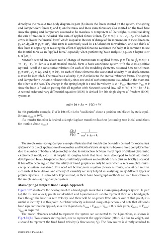
Figure 9.23 illustrates the development of a bond graph model for a mass-spring-damper system. In part
(a), the distinct velocity points are identified and 1-junctions are used to represent them on a bond graph.
Even though the base has zero velocity, and there will be no power flow into or out of that point, it is
useful to identify it at this point. A relative velocity is formed using a 0-junction, and note that all bonds
have sign convention applied, so at the 0-junction, V mass - V relative - V base = 0, which gives, V relative = V mass -
V base as required.
The model elements needed to represent the system are connected to the 1-junctions, as shown in
Fig. 9.23(b). Two sources are required, one to represent the applied force (effort, S e ) due to weight, and
a second to represent the fixed based velocity (a flow source, S f ). The flow source is directly attached to

©2002 CRC Press LLC