Page 149 - The Mechatronics Handbook

3. Make any final assignments on R elements that have not had their causality assigned through steps
1 and 2, and again propagate causality as required. Any arbitrary assignment on an R element will
indicate need for solving an algebraic equation.
4. Assign any remaining bonds arbitrarily, propagating each case as necessary.
Causality can provide information about system operation. In this sense, the bond graph provides a
picture of how inputs to a system lead to certain outputs. The use of causality with a bond graph replaces
ad hoc assignment of causal notions in a system. This type of information is also useful for understanding
how a system can be split up into modules for simulation and/or it can confirm the actual physical
boundaries of components.
Completing the assignment of causality on a bond graph will also reveal information about the
solvability of the system model. The following are key results from causality assignment.
• Causality assignment will reveal the order of the system, which is equal to the number of inde-
pendent energy storage elements (i.e., those with integral causality). The state variable (p or q)
for any such element will be a state of the system, and one first-order differential equation will be
required to describe how this state propagates through time.
• Any arbitrary assignment of causality on an R element indicates there is an algebraic loop. The
number of arbitrary assignments can be related to the number of algebraic equations required in
the model.

Developing a Mathematical Model
Mathematical models for lumped-parameter mechanical systems will take the form of coupled ordinary
differential equations or, for a linear or linearized system, transfer functions between variables of interest
and system inputs. The form of the mathematical model should match the application, and one can readily
convert between the different forms. A classical approach to developing the mathematical model will involve
applying Newton’s second law directly to each body, taking account of the forces and torques. Commonly,
the result is a second-order ordinary differential equation for each body in a system. An alternative is to
use Lagrange’s equations, and for multidimensional dynamics, where bodies may have combined transla-
tion and rotation, additional considerations are required as will be discussed in Section 9.6. At this point,
consider those systems where a given body is either under translation or rotation.

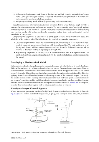
Mass-Spring-Damper: Classical Approach
A basic mechanical system that consists of a rigid body that can translate in the z-direction is shown in
Fig. 9.22(a). The system is modeled using a mass, a spring, and a damper, and a force, F(t), is applied

Rigid body, mass, m F(t) z F(t)
V
1 degree of
freedom (DOF)
dp
dt W
Spring,
F k F b
with stiffness, k Damper, with
coefficient, b

F k F b
Fixed Base (zero velocity)
V = 0

(a) (b)

FIGURE 9.22 Basic mass-spring-damper system: (a) schematic, (b) free-body diagram.

©2002 CRC Press LLC