Page 147 - The Mechatronics Handbook

The two examples in Figs. 9.20(b) and 9.20(c) demonstrate how a relative velocity can be formed. Two
masses each identify the two distinct velocity points in these systems. Using a 0-junction allows con-
struction of a velocity difference, and in each case this forms a relative velocity. In each case the relative
velocity is represented by a 1-junction, and it is critical to identify that this 1-junction is essentially an
attachment point for a basic mechanical modeling element.

Assigning and Using Causality
Bond graphs describe how modeling decisions have been made, and how model elements (R, C, etc.)
are interconnected. A power bond represents power flow, and assigning power convention using a half-
arrow is an essential part of making the graph useful for modeling. A sign convention is essential for
expressing the algebraic summation of effort and flow variables at 0- and 1-junctions. Power is generally
assigned positive sense flowing into passive elements (resistive, capacitive, inertive), and it is usually safe
to always adopt this convention. Sign convention requires consistent and careful consideration of the
reference conditions, and sometimes there may be some arbitrariness, not unlike the definition of
reference directions in a free-body diagram.
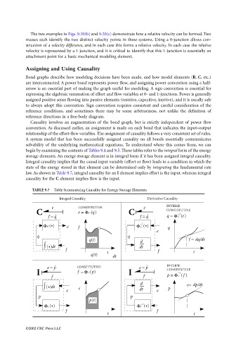
Causality involves an augmentation of the bond graph, but is strictly independent of power flow
convention. As discussed earlier, an assignment is made on each bond that indicates the input–output
relationship of the effort-flow variables. The assignment of causality follows a very consistent set of rules.
A system model that has been successfully assigned causality on all bonds essentially communicates
solvability of the underlying mathematical equations. To understand where this comes from, we can
begin by examining the contents of Tables 9.4 and 9.5. These tables refer to the integral form of the energy
storage elements. An energy storage element is in integral form if it has been assigned integral causality.
Integral causality implies that the causal input variable (effort or flow) leads to a condition in which the
state of the energy stored in that element can be determined only by integrating the fundamental rate
law. As shown in Table 9.7, integral causality for an I element implies effort is the input, whereas integral
causality for the C element implies flow is the input.

TABLE 9.7 Table Summarizing Causality for Energy Storage Elements
Integral Causality Derivative Causality

e CONSTITUTIVE e INVERSE
C e =ΦC (q) C CONSTITUTIVE
−1
f = q f = q q =ΦC (e)
−1
ΦC ( ) e f ΦC () q
e
q q
q(t) d f = dq/dt
∫ ()dt dt
f f t
q(t) t
dt
INVERSE
e = p CONSTITUTIVE e = p CONSTITUTIVE
I f =ΦI (p) I −1
f f p =ΦI (f )
d dp/dt
∫ ()dt e p e=
e dt e
p p(t) p

−1
ΦI () ΦI ()
f f
t t

©2002 CRC Press LLC