Page 143 - The Mechatronics Handbook

i f
V 1 field
i 1
ω 2 excited
θ
F 1
T 2
v 1
T 2
signal bond ω 2
conveys modulation
power
into field 1 I Field
(
m θ) circuit inductance
T 2 F 1
1 T 1 signal bond
ω 2 V 1 r(i ) conveys modulation
power v 1 f T 2
signal information is extracted from into armature
either a 1 (flow) or 0 (effort) junction circuit G
but there is no power transferred i 1 ω 2
MTF MGY
Another symbol for Another symbol for
the Modulated Transformer the Modulated GYrator
(a)
(b)
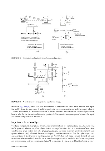
FIGURE 9.15 Concept of modulation in transformers and gyrators.
r ω 3
3
output 1 ω 3
ω r
x 2 2
2
r T:m =
F 2 2 r
3
r 1 ω 2
1
r (x )
T:m = 1 2 x 2
r
2
1 ω
ω 1
input 1
(a) (b)

FIGURE 9.16 A nonholonomic constraint in a transformer model.

model of Fig. 9.16(b), which has two transformers to represent the speed ratio between the input
(turntable) 1 and the mid-rotor 2, and the speed ratio between the mid-rotor and the output roller 3.
The first transformer is a mechanical version of a nonholonomic transformation. Specifically, we would
have to solve for the dynamics of the rotor position (x 2 ) in order to transform power between the input
and output components of this device.

Impedance Relationships
The basic component descriptions presented so far are the basis for building basic models, and a very
useful approach relies on impedance formulations. An impedance function, Z, is a ratio of effort to flow
variables at a given system port of a physical device, and the most common application is for linear
systems where Z = Z(s), where s is the complex frequency variable (sometimes called the Laplace operator).
An admittance is the inverse of the impedance, or Y = 1/Z. For each basic element defined, a linear
impedance relation can be derived for use in model development. First, recall that the derivative operator
can be represented by the s operator, so that dx/dt in s-domain is simply sx and ∫x dt is x/s, and so on.

©2002 CRC Press LLC