Page 610 - The Mechatronics Handbook

0066_Frame_C20 Page 80 Wednesday, January 9, 2002 5:49 PM

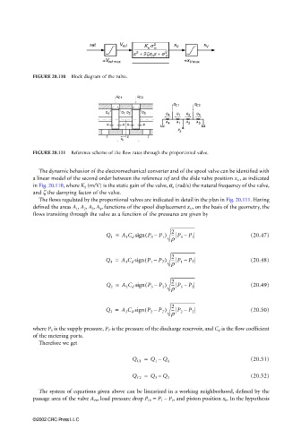
FIGURE 20.110 Block diagram of the valve.

FIGURE 20.111 Reference scheme of the flow rates through the proportional valve.

The dynamic behavior of the electromechanical converter and of the spool valve can be identified with
a linear model of the second order between the reference ref and the slide valve position x V , as indicated
in Fig. 20.110, where K S (m/V) is the static gain of the valve, σ n (rad/s) the natural frequency of the valve,
and ζ the damping factor of the valve.
The flows regulated by the proportional valves are indicated in detail in the plan in Fig. 20.111. Having
defined the areas A 1 , A 2 , A 3 , A 4 , functions of the spool displacement x V , on the basis of the geometry, the
flows transiting through the valve as a function of the pressures are given by

2
Q 1 = A 1 C d sign P S – P 1 ) --- P S – P 1 (20.47)
(
r

2
(
Q 4 = A 4 C d sign P 1 – P T ) --- P 1 – P T (20.48)
r
2
(
Q 2 = A 2 C d sign P S – P 2 ) --- P S – P 2 (20.49)
r
2
Q 3 = A 3 C d sign P 2 – P T ) --- P 2 – P T (20.50)
(
r
where P S is the supply pressure, P T is the pressure of the discharge reservoir, and C d is the flow coefficient
of the metering ports.
Therefore we get

Q C1 = Q 1 – Q 4 (20.51)

Q C2 = Q 3 – Q 2 (20.52)

The system of equations given above can be linearized in a working neighborhood, defined by the
passage area of the valve A V0 , load pressure drop P L0 = P 1 – P 2 , and piston position x 0 . In the hypothesis

©2002 CRC Press LLC