Page 988 - The Mechatronics Handbook

0066_frame_Ch33.fm Page 12 Wednesday, January 9, 2002 8:00 PM

otherwise

T
r = r R T (33.22)
T
Correction Matrix Design
∗ T ∗
The matrix F is F = A −Kc , where A is the matrix of the observer. For F the chosen poles are s 1 , s 2 ,…,
s n , and

[
det sI-F] = ( ss 1 ) ss–( 2 ) … ( ss n ) (33.23)
–
–
[
det sI-F] = s + f n−1 s n−1 + … + f 1 s + f 0 (33.24)
n
From these two equations, the coefficients k 1 , k 2 ,…, k n are obtained.
T
In this case, c = (1 0 0) and the matrix of the third observer is
 0 1 0 
∗
A =   0 0 1   (33.25)
0  – w Z 2 – 2D Z w Z 

The correction matrix influences the transient behavior; the further the poles of F from the poles of
∗
A the quicker the response.

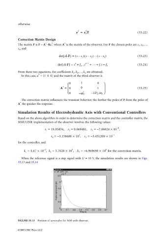
Simulation Results of Electrohydraulic Axis with Conventional Controllers
Based on the above algorithm in order to determine the correction matrix and the controller matrix, the
SIMULINK implementation of the observer involves the following values:

−4
r = 19.95854, r = 0.069481, r = −7.06024 × 10 ,
2
3
1
2 −1
r = −3.158688 × 10 , r = −3.451209 × 10
4
5
for the controller, and
6
4
−2
k = 1.67 × 10 , k = 3.7028 × 10 , k = −6.969698 × 10 for the correction matrix.
2
1
3
When the reference signal is a step signal with U = 10 V, the simulation results are shown in Figs.
33.13 and 33.14

FIGURE 33.13 Position of servovalve for MM with observer.

©2002 CRC Press LLC