
Page 452 - Thomson, William Tyrrell-Theory of Vibration with Applications-Taylor _ Francis (2010)
P. 452
Sec. 13.6 Power Spectrum and Power Spectral Density. 439
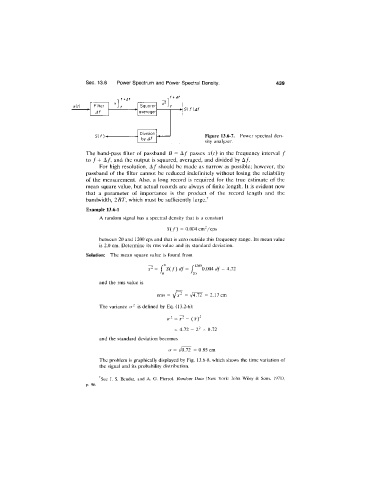
xit)
^ S { f ) A f
Figure 13.6-7. Power spectral den
sity analyzer.
The band-pass filter of passband B = passes x(t) in the frequency interval /
to / + A/, and the output is squared, averaged, and divided by A/.
For high resolution. A / should be made as narrow as possible; however, the
passband of the filter cannot be reduced indefinitely without losing the reliability
of the measurement. Also, a long record is required for the true estimate of the
mean square value, but actual records are always of finite length. It is evident now
that a parameter of importance is the product of the record length and the
bandwidth, 2BT, which must be sufficiently large.^
Example 13.6-1
A random signal has a spectral density that is a constant
S(f) = 0.004 cm^/cps
between 20 and 1200 cps and that is zero outside this frequency range. Its mean value
is 2.0 cm. Determine its rms value and its standard deviation.
Solution: The mean square value is found from
— /-oo /"1200
X^= f S{f )df = f 0.004 rf/= 4.72
•'o ■'20
and the rms value is
rms = = \/4.72 = 2.17 cm
The variance cr^ is defined by Eq. (13.2-6):
= 4.72 - 2^ = 0.72
and the standard deviation becomes
or = \/0.72 = 0.85 cm
The problem is graphically displayed by Fig. 13.6-8, which shows the time variation of
the signal and its probability distribution.
^See J. S. Bendat, and A. G. Piersol, Random Data (New York: John Wiley & Sons, 1971),
p. 96.