Page 448 - Thomson, William Tyrrell-Theory of Vibration with Applications-Taylor _ Francis (2010)

Sec. 13.6 Power Spectrum and Power Spectral Density. 435

Thus, the autocorrelation of a deflection at a given point due to separate loads
F|(0 and F2U) cannot be determined simply by adding the autocorrelations Rxir)
and Ry{r) resulting from each load acting separately, and Ry^i^) are here
referred to as cross correlation, and, in general, they are not equal.
Example 13.5-1
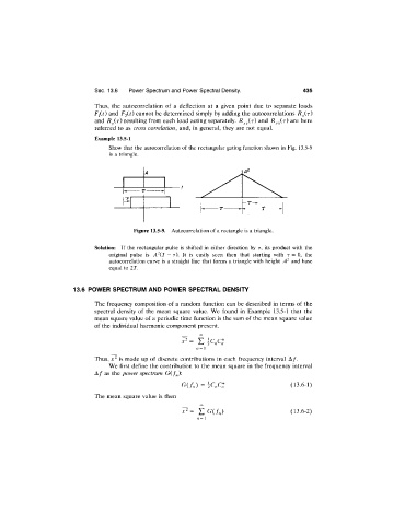
Show that the autocorrelation of the rectangular gating function shown in Fig. 13.5-9
is a triangle.

Figure 13.5-9. Autocorrelation of a rectangle is a triangle.

Solution: If the rectangular pulse is shifted in either direction by r, its product with the
original pulse is A^{T - r). It is easily seen then that starting with r = 0, the
autocorrelation curve is a straight line that forms a triangle with height and base
equal to 27.

13.6 POWER SPECTRUM AND POWER SPECTRAL DENSITY

The frequency composition of a random function can be described in terms of the
spectral density of the mean square value. We found in Example 13.5-1 that the
mean square value of a periodic time function is the sum of the mean square value
of the individual harmonic component present.
00
^ = L K « C
n = \
Thus, is made up of discrete contributions in each frequency interval A/.
We first define the contribution to the mean square in the frequency interval
A / as the power spectrum G(f^):
G { f n ) = K .Q * (13.6-1)
The mean square value is then

X^= Y. G(f„) (13.6-2)
n = l