Page 315 - Thermal Hydraulics Aspects of Liquid Metal Cooled Nuclear Reactors

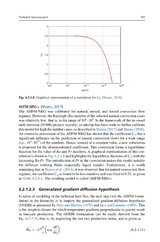
Turbulent heat transport 285

3

2.5

2

c t3 1.5

1

0.5

0
10 0 10 5 10 10 10 15 10 20
Ra*Pr
Fig. 6.2.1.8 Graphical representation of a correlation for C t3 (Shams, 2018).

AHFM-NRG+ (Shams, 2017)
The AHFM-NRG was calibrated for natural, mixed, and forced convection flow
regimes. However, the Rayleigh (Ra) number of the selected natural convection cases
4 5
was relatively low, that is, in the range of 10 –10 . In the framework of the in-vessel
melt retention (IVMR) project, recently, an attempt has been made to further calibrate
this model for high Ra number cases, as described in Shams (2017) and Shams (2018).
An extensive assessment of the AHFM-NRG has shown that the coefficient C t3 has a
significant influence on the prediction of natural convection flows for a wide range
17
3
(i.e., 10 –10 )of Ra numbers. Hence, instead of a constant value, a new correlation
is proposed for the aforementioned coefficient. This correlation forms a logarithmic
function for the value of Ra and Pr numbers. A graphical representation of this cor-
relation is shown in Fig. 6.2.1.8 and highlights the logarithmic decrease of C t3 with the
increasing Ra Pr. The introduction of Pr in the correlation makes this model suitable
for different working fluids (especially liquid metals). Furthermore, it is worth
reminding that in Shams et al. (2014), it was observed that for natural convection flow
regimes, the coefficient C t1 is found to be less sensitive and was fixed to 0.25, as given
in Table 6.2.1.1. The resulting model is called AHFM-NRG+.

6.2.1.2.3 Generalized gradient diffusion hypothesis
In terms of modeling of the turbulent heat flux, the next step (wrt the AHFM formu-
lation) in the hierarchy is to employ the generalized gradient diffusion hypothesis
(GGDH) as presented by Daly and Harlow (1970) and Ince and Launder (1989). This
is the simplest closure for which temperature gradients perpendicular to gravity result
in buoyant production. The GGDH formulation can be easily derived from the
Eq. (6.2.1.9), that is, by neglecting the last two production terms, and is given as

∂T
k
θu i ¼ C θ u i u j (6.2.1.11)
E ∂x j