Page 682 - Bird R.B. Transport phenomena

662 Chapter 21 Concentration Distributions in Turbulent Flow

will give smooth concentration profiles, provided that we use a velocity function with
continuous radial derivative, rather than the piecewise continuous expressions given in
Fig. 5.5-3. Such a function is obtainable by integrating the differential equation

(21.4-13)
dy
in the dimensionless variables v + = vjv* and y + = yv*/v of Fig. 5.5-3, with the bound-
+
ary conditions v + = 0 at \f = 0 (the wall) and dv /dy + = 0 at y + = R + (the centerline).
Equation 21.4-13 is obtained (see Problem 21B.5) by combining the cylindrical-coordinate
versions of Eqs. 5.5-3 and 5.4-4 with the dimensionless form
- exp(-y726)
forO : (21.4-14)
Vl - exp(-0.26y )
+
of the mixing-length model shown in Eq. 5.4-7. Equation 21.4-13 is solvable via the qua-
dratic formula to give
-1 + Vl +
ify >0; (21.4-15)
+
1 ify =0
and v + is then computable by quadrature using, for example, the subroutines trapzd and
qtrap of Press et al. The resulting v + function closely resembles the plotted line in Fig.
5
5.5-3, with small changes near y + = 30 where the plotted line has a slope discontinuity,
and near the centerline where the calculated v + function attains a maximum value de-
pendent on the dimensionless wall radius R + whereas the line in Fig. 5.5-3 improperly
does not.
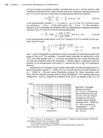
Equations 21.4-12 through 15 were solved numerically 6 for fully developed flow of a
2
fluid of kinematic viscosity v = 0.6581 cm /s in a smooth tube of 3 cm inner diameter, at
Re = 10,000, Sc = 200 and various Damkohler numbers Da. These calculations were
done with the software package Athena Visual Workbench. 7 The resulting Sherwood
numbers Sh = k D/4b ABf based on k as defined in Eq. 21.4-2, are plotted in Fig. 21.4-1 as
c
c

10,000
Fig. 21.4-1. Calculated
Sherwood numbers,
Sh = k D/4b , for turbulent
c
AB
mass transfer from the wall
1000 - •а. - 9 Ва • of a tube, with and without
Щ
^ 1 homogeneous first-order
Da = 1 J - S B chemical reaction. Results
).С calculated at Re = 10,000 and
(
( З.С I \-^ Sc = 200, as functions of
100 axial position z + = zv*/D
100 1000 10,000 and Damkohler number
Axial position, z + Da = U"vlvl.

5
W. H. Press, S. A. Teukolsky, W. T. Vettering, and B. P. Flannery, Numerical Recipes in FORTRAN,
Cambridge University Press, 2nd edition (1992).
r
' M. Caracotsios, personal communication.
7
Information on this package is available at www.athenavisual.com and from
stewartassociates.msn.com.