Page 236 - Water Engineering Hydraulics, Distribution and Treatment

214
Water Distribution Systems: Modeling and Computer Applications
Chapter 7
2.0
Continuous
Stepwise
Multiplication factor
1.5
Pump curve
Average
1.0
0.5
System curve
0.0
12
6
0
Time of day 18 24 Head Operating point H L
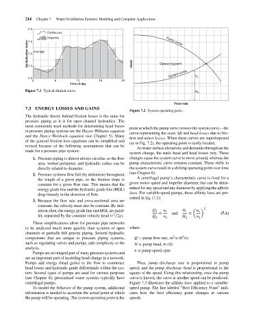
Figure 7.1 Typical diurnal curve.
H S
Flow rate
7.3 ENERGY LOSSES AND GAINS
Figure 7.2 System operating point.
The hydraulic theory behind friction losses is the same for
pressure piping as it is for open channel hydraulics. The
most commonly used methods for determining head losses
point at which the pump curve crosses the system curve—the
in pressure piping systems are the Hazen–Williams equation
curve representing the static lift and head losses due to fric-
and the Darcy–Weisbach equation (see Chapter 5). Many
tion and minor losses. When these curves are superimposed
of the general friction loss equations can be simplified and
(as in Fig. 7.2), the operating point is easily located.
revised because of the following assumptions that can be
As water surface elevations and demands throughout the
made for a pressure pipe system:
system change, the static head and head losses vary. These
1. Pressure piping is almost always circular, so the flow changes cause the system curve to move around, whereas the
area, wetted perimeter, and hydraulic radius can be pump characteristic curve remains constant. These shifts in
directly related to diameter. the system curve result in a shifting operating point over time
(see Chapter 8).
2. Pressure systems flow full (by definition) throughout
A centrifugal pump’s characteristic curve is fixed for a
the length of a given pipe, so the friction slope is
given motor speed and impeller diameter, but can be deter-
constant for a given flow rate. This means that the
mined for any speed and any diameter by applying the affinity
energy grade line and the hydraulic grade line (HGL)
laws. For variable-speed pumps, these affinity laws are pre-
drop linearly in the direction of flow.
sented in Eq. (7.1):
3. Because the flow rate and cross-sectional area are
constant, the velocity must also be constant. By defi-
( ) 2
nition, then, the energy grade line and HGL are paral- Q 1 = n 1 and H 1 = n 1 (7.1)
2
lel, separated by the constant velocity head (v ∕2g). Q 2 n 2 H 2 n 2
These simplifications allow for pressure pipe networks
to be analyzed much more quickly than systems of open where
channels or partially full gravity piping. Several hydraulic
3
3
components that are unique to pressure piping systems, Q = pump flow rate, m /s (ft /s)
such as regulating valves and pumps, add complexity to the H = pump head, m (ft)
analysis.
n = pump speed, rpm
Pumps are an integral part of many pressure systems and
are an important part of modeling head change in a network.
Pumps add energy (head gains) to the flow to counteract Thus, pump discharge rate is proportional to pump
head losses and hydraulic grade differentials within the sys- speed, and the pump discharge head is proportional to the
tem. Several types of pumps are used for various purposes square of the speed. Using this relationship, once the pump
(see Chapter 8); pressurized water systems typically have curve is known, the curve at another speed can be predicted.
centrifugal pumps. Figure 7.3 illustrates the affinity laws applied to a variable-
To model the behavior of the pump system, additional speed pump. The line labeled “Best Efficiency Point” indi-
information is needed to ascertain the actual point at which cates how the best efficiency point changes at various
the pump will be operating. The system operating point is the speeds.