Page 239 - Water Engineering Hydraulics, Distribution and Treatment

7.6 Water Quality Modeling
7.6.2 Trace Modeling
Just as a hydraulic simulation starts with some amount of
Identifying the origin of flow at a point in the system is
water in each storage tank, initial conditions must be set for a
referred to as flow tracking or trace modeling.Insystems
water age, trace, or constituent concentration analysis. These
that receive water from more than one source, trace studies
initial water quality conditions are usually unknown, so the
can be used to determine the percentage of flow from each
modeler must estimate these values from field data, a previous
source at each point in the system. These studies can be very
useful in delineating the area influenced by an individual
water quality model, or some other source of information.
source, observing the degree of mixing of water from several
To overcome the problem of unknown initial conditions
at the vast majority of locations within the water distribution
sources, and viewing changes in origins over time.
model, the duration of the analysis must be long enough
for the system to reach equilibrium conditions. Note that a
7.6.3 Constituents Modeling 7.6.4 Initial Conditions 217
constant value does not have to be reached for equilibrium to
Reactions can occur within pipes that cause the concentration be achieved; rather, equilibrium conditions are reached when
of substances to change as water travels through the system. a repeating pattern in age, trace, or constituent concentration
Based on conservation of mass for a substance within a link is established.
(for extended-period simulations only), Pipes usually reach equilibrium conditions in a short
time, but storage tanks are much slower to show a repeating
c c
= v + (c) (7.9) pattern. For this reason, extra care must be taken when setting
t x
a tank’s initial conditions, in order to ensure the model’s
where
accuracy.
c = substance concentration as a function of distance and
time 7.6.5 Numerical Methods
t = time increment
Several theoretical approaches are available for solving water
v = velocity quality models. These methods can generally be grouped as
x = distance along the link either Eulerian or Lagrangian in nature, depending on the
volumetric control approach that is taken. Eulerian models
(c) = substance rate of reaction within the link
divide the system into fixed pipe segments, and then track
the changes that occur as water flows through these seg-
In some applications, there is an additional term for
ments. Lagrangian models also break the system into con-
dispersion, but this term is usually negligible (plug flow is
trol volumes, but then track these water volumes as they
assumed through the system).
travel through the system. This chapter presents two alter-
Assuming that complete and instantaneous mixing
native approaches for performing water quality constituent
occurs at all junction nodes, additional equations can be writ-
analyses.
ten for each junction node with the following conservation
of mass equation:
Q C + Q C
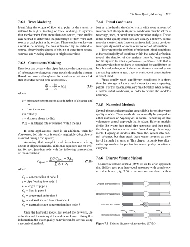
∑ 7.6.6 Discrete Volume Method
j j|x=L
e e
C k|x=0 = ∑ (7.10)
Q + Q e The discrete volume method (DVM) is an Eulerian approach
j
that divides each pipe into equal segments with completely
where
mixed volumes (Fig. 7.5). Reactions are calculated within
C = concentration at node k
k
j = pipe flowing into node k
Original concentrations
L = length of pipe j
Q = flow in pipe j
j
Reacted concentrations
C = concentration in pipe j
j
Q = external source flow into node k
e
C = external source concentration into node k Transport into nodes
e
Once the hydraulic model has solved the network, the
Transport into links
velocities and the mixing at the nodes are known. Using this
information, the water quality behavior can be derived using
a numerical method. Figure 7.5 Eulerian discrete volume method (DVM).