Page 240 - Water Engineering Hydraulics, Distribution and Treatment

218
Chapter 7
Water Distribution Systems: Modeling and Computer Applications
Original concentrations
criteria.
WaterGEMS employs a genetic algorithm search
method to find “better” solutions based on the principles of
Reacted concentrations
natural selection and biological reproduction. This genetic
algorithm program first creates a population of trial solu-
tions based on modeled parameters. The hydraulic solver
Transport through system
then simulates each trial solution to predict the HGL and
flow rates within the network and compares them to any
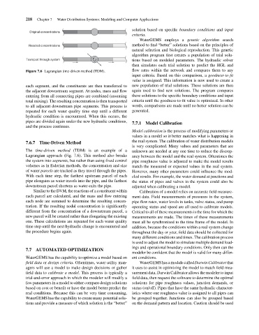
Figure 7.6 Lagrangian time-driven method (TDM).
input criteria. Based on this comparison, a goodness-to-fit
value is assigned. This information is now used to create a
new population of trial solutions. These solutions are then
each segment, and the constituents are then transferred to solution based on specific boundary conditions and input
the adjacent downstream segment. At nodes, mass and flow again used to find new solutions. The program compares
entering from all connecting pipes are combined (assuming these solutions to the specific boundary conditions and input
total mixing). The resulting concentration is then transported criteria until the goodness-to-fit value is optimized. In other
to all adjacent downstream pipe segments. This process is words, comparisons are made until no better solution can be
repeated for each water quality time step until a different generated.
hydraulic condition is encountered. When this occurs, the
pipes are divided again under the new hydraulic conditions,
7.7.1 Model Calibration
and the process continues.
Model calibration is the process of modifying parameters or
values in a model so it better matches what is happening in
the real system. The calibration of water distribution models
7.6.7 Time-Driven Method
is very complicated. Many values and parameters that are
The time-driven method (TDM) is an example of a unknown are needed at any one time to reduce the discrep-
Lagrangian approach (Fig. 7.6). This method also breaks ancy between the model and the real system. Oftentimes the
the system into segments, but rather than using fixed control pipe roughness value is adjusted to make the model results
volumes as in Eulerian methods, the concentration and size match the measured or expected values in the real system.
of water parcels are tracked as they travel through the pipes. However, many other parameters could influence the mod-
With each time step, the farthest upstream parcel of each eled results. For example, the water demand at junctions and
pipe elongates as water travels into the pipe, and the farthest the status of pipes and valves in the system could also be
downstream parcel shortens as water exits the pipe. adjusted when calibrating a model.
Similar to the DVM, the reactions of a constituent within Calibration of a model relies on accurate field measure-
each parcel are calculated, and the mass and flow entering ment data. Field measurements of pressures in the system,
each node are summed to determine the resulting concen- pipe flow rates, water levels in tanks, valve status, and pump
tration. If the resulting nodal concentration is significantly operating status and speed are all used to calibrate models.
different from the concentration of a downstream parcel, a Critical to all of these measurements is the time for which the
new parcel will be created rather than elongating the existing measurements are made. The times of these measurements
one. These calculations are repeated for each water quality must all be synchronized to the time frame of the model. In
time step until the next hydraulic change is encountered and addition, because the conditions within a real system change
the procedure begins again. throughout the day or year, field data should be collected for
many different conditions and times. The calibration process
is used to adjust the model to simulate multiple demand load-
ings and operational boundary conditions. Only then can the
7.7 AUTOMATED OPTIMIZATION
modeler be confident that the model is valid for many differ-
WaterGEMS has the capability to optimize a model based on ent conditions.
field data or design criteria. Oftentimes, water utility man- WaterGEMS has a module called Darwin Calibrator that
agers will use a model to make design decisions or gather it uses to assist in optimizing the model to match field mea-
field data to calibrate a model. This process is typically a surement data. Darwin Calibrator allows the modeler to input
trial-and-error approach in which the modeler will modify a field data, then request the software to determine the optimal
few parameters in a model to either compare design solutions solutions for pipe roughness values, junction demands, or
based on cost or benefit or have the model better predict the status (on/off). Pipes that have the same hydraulic character-
real conditions. Because this can be very time consuming, istics where one roughness value is assigned to all pipes can
WaterGEMS has the capability to create many potential solu- be grouped together. Junctions can also be grouped based
tions and provide a measure of which solution is the “better” on the demand pattern and location. Caution should be used