Page 258 - Water Engineering Hydraulics, Distribution and Treatment

236
Chapter 7
Water Distribution Systems: Modeling and Computer Applications
Color-coding range for Problem 7.3
Table 7.18
Head (ft)
Head (m)
Flow (gpm)
Max. velocity
Flow (L/min)
200
0
60.96
0
(m/s)
Color
(ft/s)
3,785
175
53.34
1,000
Magenta
0.15
0.5
7,570
100
30.48
2,000
2.5
Blue
0.76
Green
1.52
5.0
Table 7.20
Junction information for Problem 7.4
8.0
Yellow
2.44
20.0
6.10
Red
Junction Label
Demand (L/min)
400
J-1
1,514
2,082
J-2
550
Another way to quickly determine the performance of the sys- Table 7.19 Pump information for Problem 7.4 Demand (gpm)
tem is to color-code the pipes according to some indicator. J-3 2,082 550
In hydraulic design, a good performance indicator is often J-4 1,325 350
the velocity in the pipes. Pipes consistently flowing below 0.5 ft/s
(0.15 m/s) may be oversized. Pipes with velocities over 5 ft/s Table 7.21 Pipe information for Problem 7.4
(1.5 m/s) are fairly heavily stressed, and those with velocities above
8 ft/s (2.4 m/s) are usually bottlenecks in the system under that flow Pipe Length Length
pattern. Color-code the system using the ranges given in Table 7.18. label (m) (ft)
After you define the color-coding, place a legend in the drawing
P-1 23.77 78
(see Table 7.18).
P-2 12.19 40
1. Fill in or reproduce the Results Summary table after each run P-3 27.43 90
to get a feel for some of the key indicators during various P-4 11.89 39
scenarios. P-5 3.05 10
2. For the average day run, what is the pump discharge? P-6 3.05 10
3. If the pump has a best efficiency point at 300 gpm
(1,135.5 L/min), what can you say about its performance on 1. What are the resulting flows and velocities in the pipes?
an average day? 2. What are the resulting pressures at the junction nodes?
4. For the peak hour run, the velocities are fairly low. Does this 3. Place a check valve on pipe P-3 such that the valve only allows
mean you have oversized the pipes? Explain. flow from J-3 to J-4. What happens to the flow in pipe P-3?
5. For the minimum hour run, what was the highest pressure in Why does this occur?
the system? Why would you expect the highest pressure to 4. When the check valve is placed on pipe P-3, what happens to
occur during the minimum hour demand? the pressures throughout the system?
6. Was the system (as currently designed) acceptable for the fire 5. Remove the check valve on pipe P-3. Place a 6 in. (150 mm)
flow case with the sprinkled building? On what did you base flow control valve (FCV) node at an elevation of 5 ft (1.52 m)
this decision? on pipe P-3. The FCV should be set so that it only allows a
7. Was the system (as currently designed) acceptable for the flow of 100 gpm (378.5 L/min) from J-4 to J-3. (Hint: A check
fire flow case with all the flow provided by hose streams (no valve is a pipe property.) What is the resulting difference in
sprinklers)? If not, how would you modify the system so that flows in the network? How are the pressures affected?
it will work?
6. Why does not the pressure at J-1 change when the FCV is
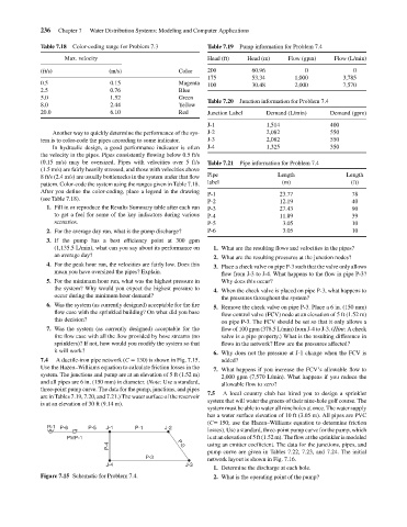
7.4 A ductile-iron pipe network (C = 130) is shown in Fig. 7.15. added?
Use the Hazen–Williams equation to calculate friction losses in the 7. What happens if you increase the FCV’s allowable flow to
system. The junctions and pump are at an elevation of 5 ft (1.52 m) 2,000 gpm (7,570 L/min). What happens if you reduce the
and all pipes are 6 in. (150 mm) in diameter. (Note: Use a standard, allowable flow to zero?
three-point pump curve. The data for the pump, junctions, and pipes
7.5 A local country club has hired you to design a sprinkler
are in Tables 7.19, 7.20, and 7.21.) The water surface of the reservoir
system that will water the greens of their nine-hole golf course. The
is at an elevation of 30 ft (9.14 m).
system must be able to water all nine holes at once. The water supply
has a water surface elevation of 10 ft (3.05 m). All pipes are PVC
(C= 150; use the Hazen–Williams equation to determine friction
R-1 P-6 P-5 J-1 P-1 J-2 losses). Use a standard, three-point pump curve for the pump, which
PMP-1 is at an elevation of 5 ft (1.52 m). The flow at the sprinkler is modeled
P-4 P-2 using an emitter coefficient. The data for the junctions, pipes, and
pump curve are given in Tables 7.22, 7.23, and 7.24. The initial
P-3 network layout is shown in Fig. 7.16.
J-4 J-3
1. Determine the discharge at each hole.
Figure 7.15 Schematic for Problem 7.4. 2. What is the operating point of the pump?