Page 253 - Water Engineering Hydraulics, Distribution and Treatment

231
7.7 Automated Optimization
the Observed Target tab. Select the junctions from the drawing by clicking the Select button then clicking junctions J-7 J-6, J-l,
and J-2 from the drawing. Click the green check in the Select dialog. Select Pressure (kPa) for each junction in the Attribute
field. Enter the measured pressure for each junction in the Value field.
Enter the tank level in the Boundary Overrides tab. Select the tank from the drawing by clicking the Select button then clicking
the tank. Click the green check in the Select dialog. Select Tank Level (m) in the Attribute field, then enter 3.93 m in the Value
field.
To make sure the pump is off, click the New buttoninthe Boundary Overrides tab. Select the pump by clicking the Select
button, then clicking the pump. Click the green check in the Select dialog. Select Pump Status in the Attribute field, then
select Off in the Value field.
Enter the additional demand at junction 7 in the Demand Adjustments tab. Select this junction from the drawing by clicking
the Select button, then clicking J-7. Click the green check in the Select dialog. Enter 3400 L/min in the Value field.
Select the pipes where the roughness values are to be determined in the Roughness Groups tab. Pipes with similar roughness
Enter the field data in the Field Data Snapshots tab. Click the New button to enter new data. Enter the measured pressures on
can be grouped together, or the software can analyze each pipe separately. In this case, the software will determine the pipe
roughness values for P-2, P-l, and P-8 separately, and pipes P-3 and P-7 will be grouped since we assume they are both 200
mm (8 in.) ductile-iron pipes, and we do not have any field measurements isolating these pipes. Click the New button, then the
Ellipse button in the Elements field. Click the select button, and then pipe P-2 from the drawing. Click the green check in the
Select dialog. Click OK to enter this pipe into the table. Repeat these steps to add pipes P-1 and P-8 to the table. You should
have three defined roughness groups in the table on the Roughness Groups tab.
Add the grouped pipes by clicking the New button, then the Ellipse buttoninthe Elements field. Click the select button, then
pipes P-3 and P-7 from the drawing. Click the green check in the Select dialog. Click OK to enter these pipes into the table as
a group. There should now be four roughness groups in the table on the Roughness Groups tab.
The calibration method settings are found on the Calibration Criteria tab. In this case, these settings will be left as the default

settings.
To use these data to determine the pipe roughness values, create a new run by clicking the New button above the left window,

then select New Optimized Run.
The pipe roughness values are assumed to have a range between 5 and 140 for each pipe. This is a wide range and any chokes

(blockages, partially closed valves, etc.) in a pipe could greatly reduce the pipe roughness value. It is not expected that any
roughness value above 140 would not be observed for ductile-iron pipe. On the Roughness tab in the Operation field, Set
should be selected; the expected minimum and maximum roughness values are entered in the Minimum Value and Maximum
Value fields. Enter the increment for the software to analyze the roughness values by entering 5 into the Increment field. Other
increments could be used.
For this simulation, the top five solutions will be displayed. To do this, click the Options tab and enter 5 into the Solutions to

Keep field.
To start the run, click the Compute button in the Darwin Calibrator toolbar. When the run is completed, close the Calibration…
window. The top five solutions will be listed under the “New Optimized Run” in the left window.
Answer
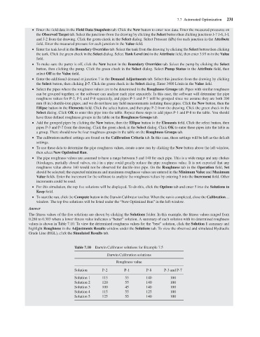
The fitness values of the five solutions are shown by clicking the Solutions folder. In this example, the fitness values ranged from
0.280 to 0.303 where a lower fitness value indicates a “better” solution. A summary of each solution with its determined roughness
values is shown in Table 7.10. To view the determined roughness values for the “best” solution, click the Solution 1 summary and
highlight Roughness in the Adjustments Results window under the Solutions tab. To view the observed and simulated Hydraulic
Grade Line (HGL), click the Simulated Results tab.
Table 7.10 Darwin Calibrator solutions for Example 7.5
Darwin Calibration solutions
Roughness value
Solution P-2 P-1 P-8 P-3 and P-7
Solution 1 115 55 140 100
Solution 2 120 55 140 100
Solution 3 100 45 140 100
Solution 4 115 55 125 100
Solution 5 125 55 140 100