Page 248 - Water Engineering Hydraulics, Distribution and Treatment

226
Water Distribution Systems: Modeling and Computer Applications
Close the options window to look at the graph. Notice that the water age in the junctions is much less (2–4 h) than the water in the
tank while the pump is on and feeding freshwater into the system. Then the water age in the junctions greatly increases when the
system is fed by the tank water after the pump turns off.
Water Quality Analysis
To analyze the behavior of chlorine in the network, the properties of chlorine must be defined in the engineering library.
From the Components menu, select Engineering Libraries. Double-click the Constituent Libraries. Then right-click on the
ConstituentLibrary.xlm to select Add Item.
Rename the new constituent by right-clicking it and selecting Rename. Change the label to “Chlorine.” Click on the Chlorine
2
dialog. Enter the Diffusivity (l.l22e–010 m /s). Enter the Bulk Reaction Order as 1 and the Bulk Reaction Rate as –0.5
1–n
–1
(mg/L)
From the Analysis menu, select Scenarios. Create a new base scenario named “Chlorine Analysis.”
Chapter 7 /day. Because n = 1, the units of the rate constant are day . Close the Engineering Libraries.
Click on the Calculation Options tab at the bottom of the window. Create a new Calculation Option by clicking the New button
and enter “Chlorine Analysis Calculation Options” as the name. Double-click the calculation options you just created and select
Constituent in the Calculation Type field. The Duration is 168 h (7 days), and the Hydraulic Time Step is 1.00 h.
Go back to the Scenarios tab and right-click the Chlorine Analysis scenario and select Make Current. The red check should
now be on the Chlorine Analysis scenario. Double-click on the Chlorine Analysis scenario and select the Chlorine Analysis
Calculation Options in the Calculation Options field.
Go to the Alternatives tab. Double-click on the Constituent; right-click on Base Constituent Alternative to select Open. Select

the Constituent System Data tab then click the ellipse button. Click the Synchronization Options button to select Import from
Library. Select Chlorine from the Constituent Libraries list. Close the Constituents dialog. Select Chlorine in the Constituent
field on the Constituents: Base Constituents Alternative window. Close the Constituent Alternative window.
Double-click the reservoir to define the loading of chlorine. Select True in the Is Constituent Source? field. The Constituent

Source Type is Concentration and the baseline concentration is 1.0 mg/L. The constituent source pattern is fixed.
The bulk reaction rate in the pipes can be adjusted using the Tables tool. Click the Flex Table button, then select the Pipe Table.

Add the Bulk Reaction Rate (Local) and Specify Local Bulk Reaction Rate? to the table by clicking the Edit button in the toolbar
at the top of the table. Scroll to the Specify Local Bulk Reaction Rate? column to click the box for the pipe you want to adjust.
Now you can enter a reaction value for the pipe in the Bulk Reaction Rate (local) column. In this case we will not change any
of the default values so close the Pipe Table.
Double-click the tank. Set the initial chlorine concentration to 0.000 mg/L, select True in the Specify Local Bulk Rate? field,

then enter the bulk reaction rate of –0.5 per day. Close the editor dialog.
From the Analysis menu, select Scenarios. Make sure Chlorine Analysis is the current scenario then run the scenario by clicking
the Compute button in the top row.
Open the EPS Results Browser window by clicking the icon button. To create a contour map of the chlorine concentration, click
the Contour button. After clicking the New button, contour by Concentration (Calculated); select all elements; set the Minimum
to 0.0, Maximum to 1.0, Increment to 0.025, and Index to 0.1 mg/L. Click the Play button on the Animation Control window.
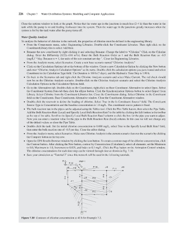
The chlorine concentrations for each time step can be viewed through time as shown in Fig. 7.10.
Save your simulation as “Tutorial 2” since this network will be used in the following tutorials.
R-1 PMP-1
P-12
J-6 P-8 P-13 P-10 J-8 J-9
J-7 P-11
P-7 P-9
P-1 J-4 P-6 J-5
J-1
P-3 P-5
P-2
J-2
P-4 J-3
P-14

T-1
Figure 7.10 Contours of chlorine concentration at 42 h for Example 7.2.