Page 249 - Water Engineering Hydraulics, Distribution and Treatment

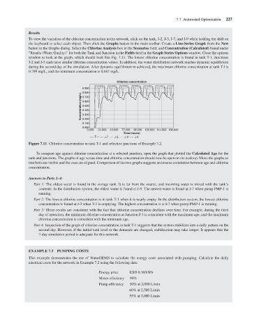
Results
To view the variation of the chlorine concentration in the network, click on the tank, J-2, J-3, J-7, and J-9 while holding the shift on
the keyboard to select each object. Then click the Graphs button in the main toolbar. Create a Line-Series Graph from the New
button in the Graphs dialog. Select the Chlorine Analysis box in the Scenarios field, and Concentration (Calculated) found under
“Results (Water Quality)” for both the Tank and Junction in the Fields field in the Graph Series Options window. Close the options
window to look at the graph, which should look like Fig. 7.11. The lowest chlorine concentration is found in tank T-1. Junctions
J-2 and J-3 each have similar chlorine concentration values. In addition, the water distribution network reaches dynamic equilibrium
during the second day of the simulation. After dynamic equilibrium in achieved, the maximum chlorine concentration at tank T-l is
0.799 mg/L, and the minimum concentration is 0.687 mg/L.
0.900 Chlorine concentration 7.7 Automated Optimization 227
0.800
Concentration (mg/L) 0.600
0.700
0.500
0.400
0.300
0.200
0.100
0.000
0.000 24.000 48.000 72.000 96.000 120.000 144.000 168.000
Time (hours)
T-1 J-7 J-2 J-9 J-3
Figure 7.11 Chlorine concentration in tank T-1 and selection junctions of Example 7.2.
To compare age against chlorine concentration at a selected junction, open the graph that plotted the Calculated Age for the
tank and junctions. The graphs of age versus time and chlorine concentration should now be open on the desktop. Move the graphs so
that both are visible and the axes are aligned. Comparison of the two graphs suggests an inverse correlation between age and chlorine
concentration.
Answers to Parts 1–4:
Part 1: The oldest water is found in the storage tank. It is far from the source, and incoming water is mixed with the tank’s
contents. In the distribution system, the oldest water is found at J-9. The newest water is found at J-7 when pump PMP-1 is
running.
Part 2: The lowest chlorine concentration is in tank T-1 when it is nearly empty. In the distribution system, the lowest chlorine
concentration is found at J-3 when T-1 is emptying. The highest concentration is at J-7 when pump PMP-1 is running.
Part 3: These results are consistent with the fact that chlorine concentration declines over time. For example, during the third
day of operation, the minimum chlorine concentration at Junction J-3 is coincident with the maximum age, and the maximum
chlorine concentration is coincident with the minimum age.
Part 4: Inspection of the graph of chlorine concentration in tank T-1 suggests that the system stabilizes into a daily pattern on the
second day. However, if the initial tank level or the demands are changed, stabilization may take longer. It appears that the
7-day simulation period is adequate for this network.

EXAMPLE 7.3 PUMPING COSTS
This example demonstrates the use of WaterGEMS to calculate the energy costs associated with pumping. Calculate the daily
electrical costs for the network in Example 7.2 using the following data:

Energy price USD 0.10/kWh
Motor efficiency 90%
Pump efficiency 50% at 2,000 L/min
60% at 2,500 L/min
55% at 3,000 L/min