Page 252 - Water Engineering Hydraulics, Distribution and Treatment

230
Chapter 7
Water Distribution Systems: Modeling and Computer Applications
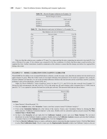
Darwin Designer solutions for Example 7.4
Darwin Designer solutions
Solution
Solution 1
217,382
Solution 2
218,687
220,548
Solution 3
Table 7.9
Pipe diameters and costs for Solution 1 of Example 7.4
Diameter (mm)
Pipe
P-3 Table 7.8 Pipe diameters and costs for Solution 1 Total cost ($) Cost ($)
250
25,812
P-10 200 23,887
P-6 200 23,887
P-14 200 23,808
P-11 200 23,808
P-8 150 17,049
P-4 150 17,049
P-9 200 15,872
P-7 150 12,744
P-2 75 12,298
P-1 75 12,096
P-5 75 9,072
Note also that this solution uses a number of 75 mm (3 in.) pipes and that the pipe connecting the network to the tank (P-14) is
only a 200 mm (8 in.) pipe. If this solution was evaluated for fire flow conditions, it is likely that these pipes would not deliver the
required fire flow. Further simulations should be conducted on this solution to ensure that this design can deliver the required flow
during a fire event.
EXAMPLE 7.5 MODEL CALIBRATION USING DARWIN CALIBRATOR
WaterGEMS has the ability to use measured field data to calibrate a model. In many cases, data that are entered into the model are an
approximation or guess. When the model results do not match field data, then parameters in the model are adjusted. Also, using the
Darwin Calibrator and field data, we can locate potential differences between the real network and the model that could be caused by
problems in the system (blockages, closed valves, etc.).
Adjust the Hazen–Williams C factor (roughness factor) for pipes P-2, P-1, and P-8 for the pipe network from Example 7.2.
During the field measurements, the tank level was 3.93 m, the pump was off, and a hydrant with a measured flow of 3400 L/min at
junction 7 (J-7) was opened to increase the head loss in the pipe network. The measured field data are shown below:
Junction Pressure (kPa)
J-7 296.0
J-6 406.5
J-1 263.5
J-2 327.0
Solution:
Open Tutorial 2 (from Example 7.2).

From the Analysis menu, select Scenarios. Create a new base scenario named “Calibrator Analysis.”

Clickonthe Calculation Options tab at the bottom of the window. Create a new Calculation Option by clicking the New
button and enter “Calibrator Calculation Options” as the name. Double-click the calculation options you just created. The Time
Analysis Type is Steady State.
Go back to the Scenarios tab and right-click the Calibrator Analysis scenario and select Make Current. The red check
should now be on the Calibrator Analysis scenario. Double-click on the Calibrator Analysis scenario and select the Calibrator
Calculation Options in the Calculation Options field. Click the Compute button.
Click the Darwin Calibrator button to create a calibration study to determine the pipe roughness factors. Click the New button
to select New Calibration Study. Check to make sure the Representative Scenario window has Calibrator Analysis selected.