Page 315 - Wind Energy Handbook

BLADE FATIGUE STRESSES 289

F Y .dr
C d . 1 / 2 pW 2 . c(r)dr
F X .dr
C l . 1 / 2 pW 2 c(r).dr

φ
O S
α
F x = (C l cos φ + C d sin φ) 1 / 2 pW 2 . c(r)
F y = (C l sin φ + C d cos φ) 1 / 2 pW 2 . c(v) W
φ
V R
M x = ∫( F y )(r-r*)dv
U r* R
Q M y = ∫(F x )(r-r*)dv
r*
M X
θ′
O S
M Y
U
V
M uu = M y cos θ' + M x sin θ'
M vv = M y sin θ' + M x cos θ'
V
M vv
U
v
M uu
P u
O S
σ′ p = –( + ) U
M uu .u M vv .v
I uu I vv V

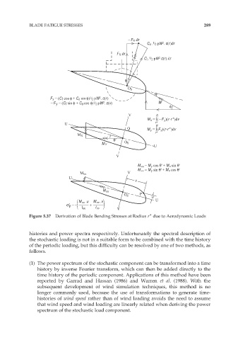
Figure 5.37 Derivation of Blade Bending Stresses at Radius r due to Aerodynamic Loads

histories and power spectra respectively. Unfortunately the spectral description of
the stochastic loading is not in a suitable form to be combined with the time history
of the periodic loading, but this difficulty can be resolved by one of two methods, as
follows.

(1) The power spectrum of the stochastic component can be transformed into a time
history by inverse Fourier transform, which can then be added directly to the
time history of the periodic component. Applications of this method have been
reported by Garrad and Hassan (1986) and Warren et al. (1988). With the
subsequent development of wind simulation techniques, this method is no
longer commonly used, because the use of transformations to generate time-
histories of wind speed rather than of wind loading avoids the need to assume
that wind speed and wind loading are linearly related when deriving the power
spectrum of the stochastic load component.