Page 285 - Adaptive Identification and Control of Uncertain Systems with Nonsmooth Dynamics

Identification and Control of Hammerstein Systems With Hysteresis Non-linearity 287

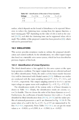
Table 18.1 Identification of the order of linear dynamics
Voltage T = 0.5 s T = 0.2 s T = 0.1 s
4V 2 3 2
5V 2 2 3

surface, which depends on the bound of disturbance to be rejected. More-
over, to reduce the chattering issue coming from the signum function, a
time-varying gain q|s(k)| depending on the value of s(k) is used in the con-
η
trol (18.29), such that the chattering issue can be suppressed when s(k) is
small. The stability of the proposed control has been proved in [22], which
will not be presented here.

18.5 SIMULATIONS

This section provides simulation results to validate the proposed identifi-
cation and control methods. In the identification, we collect input/output
data based on a turntable servo motor system, which has been described in
previous chapters of this book.

18.5.1 Identification of Linear Dynamics

The blind identification is first applied for this servo system at the open
loop operation condition. The input/output data sets are collected and used
for offline identification. Firstly, the order n of the linear transfer function
G(z) will be determined with Hankel matrix (18.5). Different case studies
are conducted with the input sampling interval T = 0.1s, T = 0.2s, and
T = 0.5 s, respectively. The output sampling interval is h = 0.1s and the
input voltage are square waves with amplitude U in = 4V, U in = 5V [22].
The identification results of the system order n of linear dynamics is
shown in Table 18.1. Clearly, the identification results are concise, i.e.,
n = 2 is feasible. Thus we choose the order of the linear dynamics as n = 2.
Furthermore, the coefficients of transfer function G(z) with n = 2can be
identified by blind identification from (18.10), (18.16) and the online pro-
files of estimated parameters a i and b i are illustrated in Fig. 18.5A–D. The
mean values of a i and b i for U in = 4V, U in = 5 V are summarized in Ta-
bles 18.2–18.4, respectively. From Tables 18.2–18.4, we can get the mean
values a 1 =−1.8024, a 2 = 0.3589, b 1 =−0.3569, b 2 =−0.0923.