Page 284 - Adaptive Identification and Control of Uncertain Systems with Nonsmooth Dynamics

286 Adaptive Identification and Control of Uncertain Systems with Non-smooth Dynamics

We denote the reference to be tracked as y r ,andlet R(k) =[y r (k),
y r (k − 1),...y r (k − n)], Y(k) =[y(k),y(k − 1),...,y(k − n)], then a sliding
mode surface is designed as

s(k) = C eR(k) − C eY(k) (18.27)

where C e =[c n−1 ,...,c,1] with c > 0 are appropriately selected parameters.
We further design a discrete reaching law as

s(k + 1) =(1 − qT)s(k) − ξTsgn(s(k))
s(k) ξT
=(1 − qT)s(k) − ξT = (1 − qT − )s(k) = ps(k)
|s(k)| |s(k)|
(18.28)

where q > 0 denotes the convergence speed of the sliding mode variable,
ξ> 0 is the gain associated with the signum function sgn(·), T is the sam-
ξT
pling period, and p = 1 − qT − .
|s(k)|
Based on the sliding surface and the inverse Preisach model (18.20), the
feedback controller can be designed as

−1
u(k) =f −1 ((C eB) [C eR(k + 1) − C eAY(k) − (1 − qT)s(k)
q|s(k)|
+ Tsgn(s(k))])
η
k
−1 (18.29)
= δ ki (C eB) [C eR(i + 1) − C eAY(i) − (1 − qT)s(i)
i=1
q|s(i)|
+ Tsgn(s(i))]
η
where η is a positive constant and δ ki denotes the element of matrix δ at k
row and i column. A,B are defined as follows:

⎡ ⎤ ⎡ ⎤
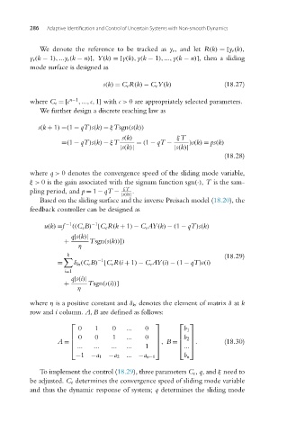
0 1 0 ... 0 b 1
⎢ 0 0 1 ... 0 ⎥ ⎢ ⎥
⎢
⎥, B = ⎢ ⎥. (18.30)
⎢b 2⎥
⎥
⎣ ... ... ... ... 1 ⎦ ⎣...⎦
A = ⎢
−1 −a 1 −a 2 ... −a n−1 b n
To implement the control (18.29), three parameters C e, q,and ξ need to
be adjusted. C e determines the convergence speed of sliding mode variable
and thus the dynamic response of system; q determines the sliding mode