Page 445 - Advanced thermodynamics for engineers

18.2 LIQUEFACTION BY EXPANSION – METHOD (II) 435

800

Higher inversion temperature
T / K
600 Cooling always occurs
Inversion temperature, 400 in this region

200
Lower inversion temperature

0
0 50 100 150 200 250 300 350
Pressure / bar

FIGURE 18.9
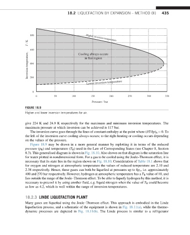
Higher and lower inversion temperatures for air.

give 224 K and 24.9 K respectively for the maximum and minimum inversion temperatures. The
maximum pressure at which inversion can be achieved is 117 bar.
The inversion curve goes through the lines of constant enthalpy at the point where (vT/vp) h ¼ 0. To
the left of the inversion curve cooling always occurs; to the right heating or cooling occurs depending
on the values of the pressure.
Figure 18.9 may be drawn in a more general manner by replotting it in terms of the reduced
pressure (p R ) and temperature (T R ) used in the Law of Corresponding States (see Chapter 8, Section
8.3). This generalised diagram is shown in Fig. 18.10. Also shown on that diagram is the saturation line
for water plotted in nondimensional form. For a gas to be cooled using the Joule–Thomson effect, it is
necessary that its state lies in the region shown on Fig. 18.10. Consideration of Table 18.1 shows that
for oxygen and nitrogen at atmospheric temperature the values of reduced temperature are 2.10 and
2.38 respectively. Hence, these gases can both be liquefied at pressures up to 8p c , i.e. approximately
400 and 270 bar respectively. However, hydrogen at atmospheric temperature has a T R value of 10, and
lies outside the range of the Joule–Thomson effect. To be able to liquefy hydrogen by this method, it is
necessary to precool it by using another fluid, e.g. liquid nitrogen when the value of T R could become
as low as 4.2, which is well within the range of inversion temperatures.

18.2.3 LINDE LIQUEFACTION PLANT
Many gases are liquefied using the Joule–Thomson effect. This approach is embodied in the Linde
liquefaction process, and a schematic of the equipment is shown in Fig. 18.11(a), while the thermo-
dynamic processes are depicted in Fig. 18.11(b). The Linde process is similar to a refrigerator