Page 89 - Advances in Biomechanics and Tissue Regeneration

84 5. IMPACT OF THE FLUID-STRUCTURE INTERACTION MODELING ON THE HUMAN VESSEL HEMODYNAMICS

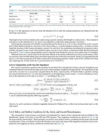
TABLE 5.1 Parameters Used to Describe the Structured Tree
Level Radius [μm] α β ξ γ η
Small arteries 250 < r 0.895 0.566 2.5 0.4 1.12
Resistance vessels 50 < r < 250 0.864 0.67 2.76 0.6 1.20
Capillaries r < 50 0.807 0.766 2.90 0.9 1.24
Notes: The binary network is divided into three levels as a function of the vessel radius. For each level, the main parameters, such as, for instance, the power exponent ξ
and the asymmetry ratio γ, were varied.

In Eq. (5.5), the exponent ξ is known from the literature [26] so that the scaling parameters are obtained from the
following expressions:
α ¼ð1+ γ ξ=2 1=ξ , β ¼ α γ: (5.6)
p
ffiffiffi
Þ
The length of each vessel is related to the radius using a special constant called length-to-radius ratio l rr . This constant is
well known in the literature [24, 27], and it was adjusted to control the outlet pressure waveform.
Following the extension of the Olufsen model performed by Steele et al. [27], we have divided the entire vascular
bed in three different levels as a function of the vessel radius r root and the length-to-radius ratio l rr , to mimic in more
detail the structure of the human circulatory system. For each level, the parameters describing the asymmetry ratio γ
and the exponent ξ were varied. The minimum radius was set to 3 μm where, as aforementioned, the blood pressure
was set to 0. Table 5.1 shows the parameters used to describe each fractal tree (one for each outlet of the two models).
Different values of l rr can be found in the literature. Based on the studies of Iberall et al. [28] on small arteries, Oluf-
sen used the value 50 while Steele used a multilevel approach also followed in this study. Zamir [29] suggested that the
mean l rr is 20 with a maximum of 70. Other studies showed that this parameter widely varies in the vascular tree, being
also organ-specific. In this work, the l rr pair has been set to 75/25 [27].

5.2.3.4 Computation of the Vascular Impedance
The vascular impedance represents the resistance to the blood flow through the vascular network. Impedance was
computed from the structured tree and used as the outlet boundary condition for large arteries. The impedance at the
root of the vascular tree is recursively computed from the linear, axisymmetric, 1D Navier-Stokes equations starting
from the terminal branch [24, 27]. The input impedance at the beginning of each vessel z ¼ 0 was evaluated as a func-
tion of the impedance at the end of a vessel z ¼ L according to Eq. (5.7):
ig 1 sinðωL=cÞ + ZðL,ωÞcosðωL=cÞ
, (5.7)
Zð0,ωÞ¼
cosðωL=cÞ + igZðL,ωÞsinðωL=cÞ
p ffiffiffiffiffiffiffiffiffiffiffiffiffiffiffiffiffiffiffiffiffiffiffiffiffiffiffiffiffiffiffi
s 0 ð1 F J Þ=ðρCÞ is the wave-propagation velocity, and
where L is the vessel length, c ¼
8μl rr 2J 1 ðw 0 Þ
, (5.8)
Zð0,0Þ¼ lim Zð0,ωÞ¼ 3 + ZðL,0Þ, F J ¼
ω!0 πr 0 w m J 0 ðw 0 Þ
2
2
3
where J 0 (x) and J 1 (x) are the zeroth- and the first-order Bessel functions with w 0 ¼ i w and w ¼r 0 ω/ν. The compliance
C can be estimated through the following equation:
Eh
3A 0 r 0
, ¼ k 1 expðk 2 r 0 Þ + k 3 , (5.9)
2Eh r 0
C ¼
where k 1 , k 2 , and k 3 are known constants originally obtained by Olufsen [25], s 0 is the cross-sectional area, and r 0 is the
root vessel.
5.2.4 Inflow and Outflow Conditions for the Aortic and Carotid Hemodynamics

The computation of the pressure waveforms was performed by means of the commercial software MatLab (The
MathWorks, Natick, MA) prior to the FSI and CFD analyses. The computed waveforms are shown in Fig. 5.3 for
the aorta and the carotid artery. These pressure waveforms were used as outflow conditions for the aortic and carotid
hemodynamics. Flow waveforms found in the literature and used as the input of the impedance-based recursive com-
putations were applied as inflow conditions in both cases (see Fig. 5.3).

I. BIOMECHANICS