Page 91 - Advances in Biomechanics and Tissue Regeneration

86 5. IMPACT OF THE FLUID-STRUCTURE INTERACTION MODELING ON THE HUMAN VESSEL HEMODYNAMICS

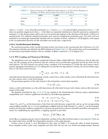
TABLE 5.3 Material Constants of the SEDF Developed in Kiousis et al. [36] Used for Modeling the
Adventitia, the Media, and the Intima Layer of the Carotid Artery
μ [kPa] k 1 [kPa] k 2 [2] ρ [2]
Adventitia 0.44 0.146 105 0.8
Media 0.7 0.023 16.9 0.8
Intima 0.7 0.023 16.9 0.8

where μ > 0 and k > 0 are stress-like parameters. k 2 > 0 and 0 ρ 1 are dimensionless parameters (when ρ ¼ 1 the
fibers are perfectly aligned and when ρ ¼ 0 the fibers are randomly distributed so that the material is considered as
isotropic), I 1 is the first invariant, and I 4 and I 6 are invariants that depend on the direction of the family of fibers at a
material point. Two different material parameters were used for modeling the presented cases. The aortic wall was
modeled as an anisotropic hyperelastic material with two families of fibers, oriented at 30.28 degrees, with respect
to the circumferential direction, for the adventitia and media layer, respectively.

5.2.8.2 Carotid Structural Modeling
The material properties of the carotid structural model were based on the experimental data of Kiousis et al. [36].
The material constants were fitted by the SEDF defined in [36] (see Table 5.3). The carotid artery wall was modeled as
an anisotropic hyperelastic material with two families of fibers, oriented at 17.22 degrees [36].

5.2.9 FSI Coupling and Numerical Modeling

The simulations were run using the commercial software Adina (Adina R&D Inc., Watertown, MA). In this soft-
ware, the FSI coupling can be performed after the creation of two models that separately include the fluid and the
solid domain. The fluid domain was solved using a standard ALE formulation [37] while the solid domain used a
typical Lagrangian formulation [38, 39]. Taking into account the moving reference velocity, the Navier-Stokes equa-
tions for the fluid domain become
B
ρ F ∂v F + ρððv F wÞ rÞv F r σ F ¼ f , (5.13)
F
∂t
B
where the term w denotes the moving mesh velocity vector [38], v F is the velocity vector of the fluid, f is the body force
F
per unit volume, and ρ F is the fluid density.
The governing equation of the solid domain is the momentum conservation equation:
B
r σ S + f ¼ ρ € u S , (5.14)
S
S
B
where ρ S is the solid density, σ S is the solid stress tensor, f is the body force per unit volume, and € u s is the local accel-
S
eration of the solid.
The domains described by Eqs. (5.13), (5.14) are coupled in the aforementioned software using a displacement
compatibility and a traction equilibrium described by the following equations:
u S ¼ u F ðx,y,zÞ2 Γ F \Γ S , (5.15)
wall wall
σ S n S + σ F n F ¼ 0 ðx,y,zÞ2 Γ F \Γ S , (5.16)
wall wall
where Γ F wall and Γ S wall are the boundaries of the fluid and solid domains, respectively, and n S , n F the corresponding
outer-pointing normals. Eq. (5.16) is an equilibrium condition between both domains Γ F wall and Γ S wall on the boundary
surfaces. Because this condition is applied in weak form, the grids between the two domains can but are not required to
match. For establishing the equilibrium, a mapping equation is provided:
Z
S T
ðH Þ M sf τ f dS, (5.17)
F S ðv,pÞ¼
where M sf is a mapping operator used to interpolate variables at the solid and fluid nodes or vice versa [38, 39], F S are
S
the solid nodal forces, and H the interpolation functions of the solid elements.
Cardiac cycles of about 1 s were discretized in time steps of 0.0001 s. To dump the effect of initial transients,
three complete cardiac cycles were computed and data from the last one was stored and postprocessed. Because

I. BIOMECHANICS