Page 239 - Applied Statistics And Probability For Engineers

c06.qxd 5/14/02 9:54 M Page 200 RK UL 6 RK UL 6:Desktop Folder:TEMP WORK:MONTGOMERY:REVISES UPLO D CH114 FIN L:Quark Files:

200 CHAPTER 6 RANDOM SAMPLING AND DATA DESCRIPTION

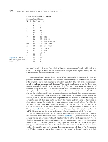
Character Stem-and-Leaf Display
Stem-and-leaf of Strength
N = 80 Leaf Unit = 1.0
1 7 6
2 8 7
3 9 7
5 10 1 5
8 11 0 5 8
11 12 0 1 3
17 13 1 3 3 4 5 5
25 14 1 2 3 5 6 8 9 9
37 15 0 0 1 3 4 4 6 7 8 8 8 8
(10) 16 0 0 0 3 3 5 7 7 8 9
33 17 0 1 1 2 4 4 5 6 6 8
23 18 0 0 1 1 3 4 6
16 19 0 3 4 6 9 9
10 20 0 1 7 8
6 21 8
Figure 6-6 A stem- 5 22 1 8 9
and-leaf diagram from 2 23 7
Minitab. 1 24 5

adequately displays the data. Figure 6-5(c) illustrates a stem-and-leaf display with each stem
divided into five parts. There are too many stems in this plot, resulting in a display that does
not tell us much about the shape of the data.

Figure 6-6 shows a stem-and-leaf display of the compressive strength data in Table 6-2
produced by Minitab. The software uses the same stems as in Fig. 6-4. Note also that the com-
puter orders the leaves from smallest to largest on each stem. This form of the plot is usually
called an ordered stem-and-leaf diagram. This is not usually done when the plot is con-
structed manually because it can be time consuming. The computer adds a column to the left of
the stems that provides a count of the observations at and above each stem in the upper half of
the display and a count of the observations at and below each stem in the lower half of the dis-
play. At the middle stem of 16, the column indicates the number of observations at this stem.
The ordered stem-and-leaf display makes it relatively easy to find data features such as per-
centiles, quartiles, and the median. The sample median is a measure of central tendency that
divides the data into two equal parts, half below the median and half above. If the number of
observations is even, the median is halfway between the two central values. From Fig. 6-6
we find the 40th and 41st values of strength as 160 and 163, so the median is
1160 1632 2 161.5. If the number of observations is odd, the median is the central value.
The sample mode is the most frequently occurring data value. Figure 6-6 indicates that the mode
is 158; this value occurs four times, and no other value occurs as frequently in the sample.
We can also divide data into more than two parts. When an ordered set of data is divided
into four equal parts, the division points are called quartiles. The first or lower quartile, q 1 , is
a value that has approximately 25% of the observations below it and approximately 75% of
the observations above. The second quartile, q 2 , has approximately 50% of the observations
below its value. The second quartile is exactly equal to the median. The third or upper quar-
tile, q 3 , has approximately 75% of the observations below its value. As in the case of the
median, the quartiles may not be unique. The compressive strength data in Fig. 6-6 contains
n 80 observations. Minitab software calculates the first and third quartiles as the 1n 12 4