Page 243 - Applied Statistics And Probability For Engineers

c06.qxd 5/14/02 9:55 M Page 204 RK UL 6 RK UL 6:Desktop Folder:TEMP WORK:MONTGOMERY:REVISES UPLO D CH114 FIN L:Quark Files:

204 CHAPTER 6 RANDOM SAMPLING AND DATA DESCRIPTION

observations. The last row of Table 6-4 expresses the relative frequencies on a cumulative ba-
sis. Frequency distributions are often easier to interpret than tables of data. For example, from
Table 6-4 it is very easy to see that most of the specimens have compressive strengths between
130 and 190 psi and that 97.5 percent of the specimens fail below 230 psi.
The histogram is a visual display of the frequency distribution. The stages for construct-
ing a histogram follow.

Constructing a
Histogram (Equal (1) Label the bin (class interval) boundaries on a horizontal scale.
Bin Widths)
(2) Mark and label the vertical scale with the frequencies or the relative
frequencies.
(3) Above each bin, draw a rectangle where height is equal to the frequency (or rel-
ative frequency) corresponding to that bin.

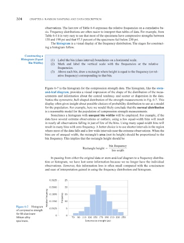
Figure 6-7 is the histogram for the compression strength data. The histogram, like the stem-
and-leaf diagram, provides a visual impression of the shape of the distribution of the meas-
urements and information about the central tendency and scatter or dispersion in the data.
Notice the symmetric, bell-shaped distribution of the strength measurements in Fig. 6-7. This
display often gives insight about possible choices of probability distribution to use as a model
for the population. For example, here we would likely conclude that the normal distribution
is a reasonable model for the population of compression strength measurements.
Sometimes a histogram with unequal bin widths will be employed. For example, if the
data have several extreme observations or outliers, using a few equal-width bins will result
in nearly all observations falling in just of few of the bins. Using many equal-width bins will
result in many bins with zero frequency. A better choice is to use shorter intervals in the region
where most of the data falls and a few wide intervals near the extreme observations. When the
bins are of unequal width, the rectangle’s area (not its height) should be proportional to the
bin frequency. This implies that the rectangle height should be
bin frequency
Rectangle height
bin width

In passing from either the original data or stem-and-leaf diagram to a frequency distribu-
tion or histogram, we have lost some information because we no longer have the individual
observations. However, this information loss is often small compared with the conciseness
and ease of interpretation gained in using the frequency distribution and histogram.

0.3125 25

0.2500 20
Relative frequency 0.1895 Frequency 15

10
0.1250
Figure 6-7 Histogram
0.0625 5
of compressive strength
for 80 aluminum-
0 0
lithium alloy 70 90 110 130 150 170 190 210 230 250
specimens. Compressive strength (psi)