Page 242 - Applied Statistics And Probability For Engineers

c06.qxd 5/14/02 12:51 PM Page 203 RK UL 6 RK UL 6:Desktop Folder:TEMP WORK:MONTGOMERY:REVISES UPLO D CH 1 14 FIN L:Quark Files:

6-4 FREQUENCY DISTRIBUTIOINS AND HISTOGRAMS 203

(b) Compute the sample mean, sample standard deviation, (b) Compute the sample mean, sample standard deviation,
and the sample median. and the sample median.
(c) A wine rated above 90 is considered truly exceptional. 6-29. A Comparative Stem-and-Leaf Diagram. In
What proportion of the taste-tasters considered this partic- Exercise 6-22, we presented height data that was self-reported
ular pinot noir truly exceptional? by female undergraduate engineering students in a core course
6-28. In their book Introduction to Linear Regression at ASU. In the same class, the male students self-reported their
Analysis (3rd edition, Wiley, 2001) Montgomery, Peck, and heights as follows:
Vining present measurements on NbOCl 3 concentration from
69 67 69 70 65 68 69 70 71 69 66 67 69 75 68 67 68
a tube-flow reactor experiment. The data, in gram mole per
3
liter 10 , are as follows: 69 70 71 72 68 69 69 70 71 68 72 69 69 68 69 73 70
73 68 69 71 67 68 65 68 68 69 70 74 71 69 70 69
450 450 473 507 457 452 453 1215 1256
1145 1085 1066 1111 1364 1254 1396 1575 1617 (a) Construct a comparative stem-and-leaf diagram by listing
the stems in the center of the display and then placing the
1733 2753 3186 3227 3469 1911 2588 2635 2725
female leaves on the left and the male leaves on the right.
(a) Construct a stem-and-leaf diagram for this data and com- (b) Comment on any important features that you notice in this
ment on any important features that you notice. display.

6-4 FREQUENCY DISTRIBUTIONS AND HISTOGRAMS

A frequency distribution is a more compact summary of data than a stem-and-leaf diagram.
To construct a frequency distribution, we must divide the range of the data into intervals, which
are usually called class intervals, cells, or bins. If possible, the bins should be of equal width
in order to enhance the visual information in the frequency distribution. Some judgment must
be used in selecting the number of bins so that a reasonable display can be developed. The num-
ber of bins depends on the number of observations and the amount of scatter or dispersion in
the data. A frequency distribution that uses either too few or too many bins will not be inform-
ative. We usually find that between 5 and 20 bins is satisfactory in most cases and that the num-
ber of bins should increase with n. Choosing the number of bins approximately equal to the
square root of the number of observations often works well in practice.
A frequency distribution for the comprehensive strength data in Table 6-2 is shown in
Table 6-4. Since the data set contains 80 observations, and since 180 9 , we suspect that
about eight to nine bins will provide a satisfactory frequency distribution. The largest and
smallest data values are 245 and 76, respectively, so the bins must cover a range of at least
245 76 169 units on the psi scale. If we want the lower limit for the first bin to begin
slightly below the smallest data value and the upper limit for the last bin to be slightly above
the largest data value, we might start the frequency distribution at 70 and end it at 250. This is
an interval or range of 180 psi units. Nine bins, each of width 20 psi, give a reasonable
frequency distribution, so the frequency distribution in Table 6-4 is based on nine bins.
The second row of Table 6-4 contains a relative frequency distribution. The relative
frequencies are found by dividing the observed frequency in each bin by the total number of

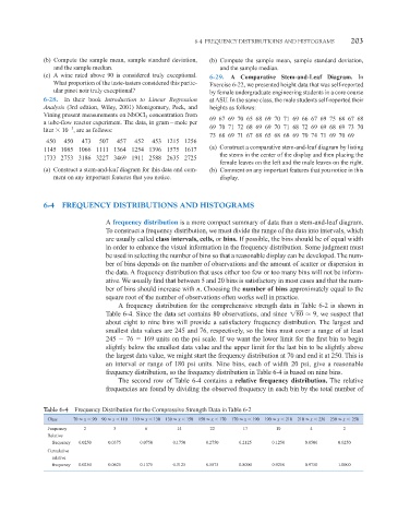
Table 6-4 Frequency Distribution for the Compressive Strength Data in Table 6-2
Class 70 x 90 90 x 110 110 x 130 130 x 150 150 x 170 170 x 190 190 x 210 210 x 230 230 x 250
Frequency 2 3 6 14 22 17 10 4 2
Relative
frequency 0.0250 0.0375 0.0750 0.1750 0.2750 0.2125 0.1250 0.0500 0.0250
Cumulative
relative
frequency 0.0250 0.0625 0.1375 0.3125 0.5875 0.8000 0.9250 0.9750 1.0000