Page 196 - Applied Statistics Using SPSS, STATISTICA, MATLAB and R

5.1 Inference on One Population 177

0
.
.
s = npq = 224 × 75 × 25 = 6.48.
0

Hence, using the continuity correction, we obtain z = (168 – 176 + 0.5)/6.48 =
−1.157, to which corresponds a one-tailed probability of 0.124 as reported in
Table 5.3.

Example 5.4
Q: Consider the Freshme n dataset, relative to the Porto Engineering College.
Assume that this dataset represents a random sample of the population of freshmen
in the College. Does this sample support the hypothesis that there is an even
chance that a freshman in this College can be either male or female?
A: We formalise the test as:

H 0: P(ω =1) = ½;
H 1: P(ω =1) ≠ ½.

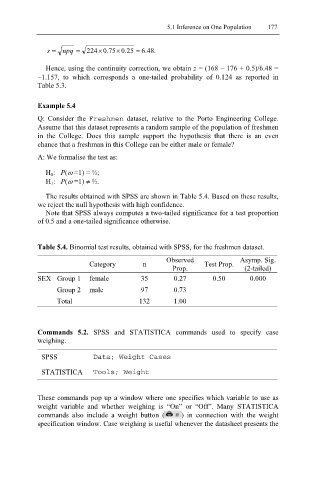
The results obtained with SPSS are shown in Table 5.4. Based on these results,
we reject the null hypothesis with high confidence.
Note that SPSS always computes a two-tailed significance for a test proportion
of 0.5 and a one-tailed significance otherwise.

Table 5.4. Binomial test results, obtained with SPSS, for the freshmen dataset.
Observed Asymp. Sig.
Category n Test Prop.
Prop. (2-tailed)
SEX Group 1 female 35 0.27 0.50 0.000
Group 2 male 97 0.73
Total 132 1.00

Commands 5.2. SPSS and STATISTICA commands used to specify case
weighing.

SPSS Data; Weight Cases

STATISTICA Tools; Weight

These commands pop up a window where one specifies which variable to use as
weight variable and whether weighing is “On” or “Off”. Many STATISTICA
commands also include a weight button ( ) in connection with the weight
specification window. Case weighing is useful whenever the datasheet presents the