Page 197 - Applied Statistics Using SPSS, STATISTICA, MATLAB and R

178 5 Non-Parametric Tests of Hypotheses

data in a compact way, with a specific column containing the number of
occurrences of each case.

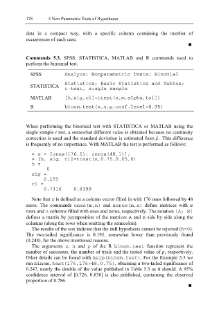
Commands 5.3. SPSS, STATISTICA, MATLAB and R commands used to
perform the binomial test.

SPSS Analyze; Nonparametric Tests; Binomial

STATISTICA Statistics; Basic Statistics and Tables;
t-test, single sample
MATLAB [h,sig,ci]=ttest(x,m,alpha,tail)
R binom.test(x,n,p,conf.level=0.95)

When performing the binomial test with STATISTICA or MATLAB using the
single sample t test, a somewhat different value is obtained because no continuity
correction is used and the standard deviation is estimated from p ˆ . This difference
is frequently of no importance. With MATLAB the test is performed as follows:

» x = [ones(176,1); zeros(48,1)];
» [h, sig, ci]=ttest(x,0.75,0.05,0)
h =
0
sig =
0.195
ci =
0.7316 0.8399

Note that x is defined as a column vector filled in with 176 ones followed by 48
zeros. The commands ones(m,n) and zeros(m,n) define matrices with m
rows and n columns filled with ones and zeros, respectively. The notation [A; B]
defines a matrix by juxtaposition of the matrices A and B side by side along the
columns (along the rows when omitting the semicolon).
The results of the test indicate that the null hypothesis cannot be rejected ( h=0 ).
The two-tailed significance is 0.195, somewhat lower than previously found
(0.248), for the above mentioned reasons.
The arguments x , n and p of the R bi nom.test function represent the
number of successes, the number of trials and the tested value of p, respectively.
Other details can be found with help(binom.test) . For the Example 5.3 we
run binom.t est(176,176+48,0.75) , obtaining a two-tailed significance of
0.247, nearly the double of the value published in Table 5.3 as it should. A 95%
confidence interval of [0.726, 0.838] is also published, containing the observed
proportion of 0.786.