Page 201 - Applied Statistics Using SPSS, STATISTICA, MATLAB and R

182 5 Non-Parametric Tests of Hypotheses

these intervals, under the “z-Interval” heading, which can be obtained from the
tables of the standard normal distribution or using software functions, such as the
ones already described for SPSS, STATISTICA, MATLAB and R.
The corresponding interval cutpoints, x cut, for the random variable under
analysis, X, can now be easily determined, using:

x cut = x + z cut s , 5.9
X

where we use the sample mean and standard deviation as well as the cutpoints
determined for the normal distribution, z cut. In the present case, the mean and
standard deviation are 137 and 43, respectively, which leads to the intervals under
the “ART-Interval” heading.
The absolute frequency columns are now easily computed. With SPSS,
*2
STATISTICA and R we now obtain the value of χ = 2.2. We must be careful,
however, when obtaining the corresponding significance in this application of the
chi-square test. The problem is that now we do not have df = k – 1 degrees of
freedom, but df = k – 1 – n p, where n p is the number of parameters computed from
the sample. In our case, we derived the interval boundaries using the sample mean
and sample standard deviation, i.e., we lost two degrees of freedom. Therefore, we
have to compute the probability using df = 5 – 1 – 2 = 2 degrees of freedom, or
equivalently, compute the critical region boundary as:

χ 2 . 0 , 2 95 = . 5 99 .

*2
Since the computed value of the χ is smaller than this critical region boundary,
we do not reject at 5% significance level the null hypothesis of variable ART being
normally distributed.

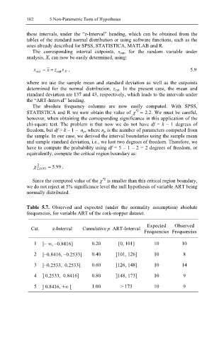
Table 5.7. Observed and expected (under the normality assumption) absolute
frequencies, for variable ART of the cork-stopper dataset.
Expected Observed
Cat. z-Interval Cumulative p ART-Interval
Frequencies Frequencies

1 ]− ∞, −0.8416] 0.20 [0, 101] 10 10

2 ]− 0.8416, −0.2533] 0.40 ]101, 126] 10 8
3 ]− 0.2533, 0.2533] 0.60 ]126, 148] 10 14

4 ] 0.2533, 0.8416] 0.80 ]148, 173] 10 9

5 ] 0.8416, + ∞ [ 1.00 > 173 10 9